Page 97 - Autonomous Mobile Robots

80 Autonomous Mobile Robots

(b) Indoor stadium
Const. threshold
60
on raw data
Threshold on
probability data
40

20
Y distance (m) 0

–20

–40

–80 –60 –40 –20 0 20 40 60
X distance (m)

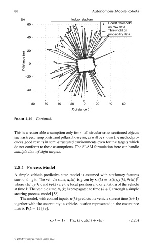
FIGURE 2.20 Continued.

This is a reasonable assumption only for small circular cross sectioned objects
such as trees, lamp posts, and pillars, however, as will be shown the method pro-
duces good results in semi-structured environments even for the targets which
do not conform to these assumptions. The SLAM formulation here can handle
multiple line-of-sight targets.

2.8.1 Process Model
A simple vehicle predictive state model is assumed with stationary features
T
surrounding it. The vehicle state, x v (k) is given by x v (k) =[x(k), y(k), θ R (k)]
where x(k), y(k), and θ R (k) are the local position and orientation of the vehicle
at time k. The vehicle state, x v (k) is propagated to time (k+1) through a simple
steering process model [38].
The model, with control inputs, u(k) predicts the vehicle state at time (k+1)
together with the uncertainty in vehicle location represented in the covariance
matrix P(k + 1) [39].

x v (k + 1) = f(x v (k), u(k)) + v(k) (2.23)

© 2006 by Taylor & Francis Group, LLC

FRANKL: “dk6033_c002” — 2006/3/31 — 17:29 — page 80 — #40