Page 98 - Autonomous Mobile Robots

Millimeter Wave RADAR Power-Range Spectra Interpretation 81

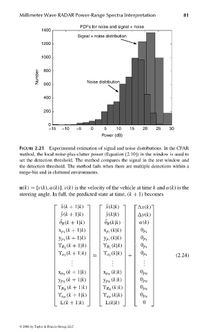
PDFs for noise and signal + noise
1400
Signal + noise distribution
1200

1000

Number 800 Noise distribution

600

400

200

0
–15 –10 –5 0 5 10 15 20 25 30
Power (dB)

FIGURE 2.21 Experimental estimation of signal and noise distributions. In the CFAR
method, the local noise-plus-clutter power (Equation [2.10]) in the window is used to
set the detection threshold. The method compares the signal in the test window and
the detection threshold. The method fails when there are multiple detections within a
range-bin and in cluttered environments.

u(k) =[v(k), α(k)]. v(k) is the velocity of the vehicle at time k and α(k) is the
steering angle. In full, the predicted state at time, (k + 1) becomes

ˆ x(k + 1|k) ˆ x(k|k) x(k)
⎡ ⎤ ⎡ ⎤ ⎡ ⎤
⎢ ˆ y(k + 1|k) ⎥ ⎢ ˆ y(k|k) ⎥ ⎢ y(k) ⎥
⎢ ⎥ ⎢ ⎥ ⎢ ⎥
ˆ ˆ
⎢ ⎥ ⎢ ⎥ ⎢ ⎥
⎢ θ R (k + 1|k) ⎥ ⎢ θ R (k|k) ⎥ ⎢ α(k) ⎥
⎢ ⎥ ⎢ ⎥ ⎢ ⎥
(k + 1|k) ⎥ (k|k) ⎥
⎢ x p 1 ⎢ x p 1 ⎢ 0 p 1 ⎥
⎢ ⎥ ⎢ ⎥ ⎢ ⎥
y (k + 1|k) y (k|k)
⎢ ⎥ ⎢ ⎥ ⎢ ⎥
⎢ p 1 ⎥ ⎢ p 1 ⎥ ⎢ 0 p 1 ⎥
⎢ ⎥ ⎢ ⎥ ⎢ ⎥
⎢ϒ R 1 (k + 1|k)⎥ ⎢ϒ R 1 (k|k)⎥ ⎢ 0 p 1 ⎥
⎢ ⎥ ⎢ ⎥ ⎢ ⎥
(2.24)
(k + 1|k) ⎥ (k|k) ⎥
⎢ ϒ a 1 ⎢ ϒ a 1 ⎢ 0 p 1 ⎥
⎢ ⎥ = ⎢ ⎥ + ⎢ ⎥
. . .
⎢ . ⎥ ⎢ . ⎥ ⎢ . ⎥
. . .
⎢ ⎥ ⎢ ⎥ ⎢ ⎥
⎢ ⎥ ⎢ ⎥ ⎢ ⎥
⎢ ⎥ ⎢ ⎥ ⎢ ⎥
⎢ x p N (k + 1|k) ⎥ ⎢ x p N (k|k) ⎥ ⎢ 0 p N ⎥
⎢ ⎥ ⎢ ⎥ ⎢ ⎥
(k + 1|k) (k|k)
⎢ ⎥ ⎢ ⎥ ⎥
y p N y p N ⎢ 0 p N ⎥
⎢ ⎥ ⎢ ⎥ ⎢
⎢ ⎥ ⎢ ⎥ ⎢ ⎥
⎢ ϒ R N (k + 1|k) ⎥ ⎢ ϒ R N (k|k) ⎥ ⎢ 0 p N ⎥
⎢ ⎥ ⎢ ⎥ ⎢ ⎥
⎣ϒ a N (k + 1|k)⎦ ⎣ϒ a N (k|k)⎦ ⎣ 0 p N ⎦
L(k + 1|k) L(k|k) 0
© 2006 by Taylor & Francis Group, LLC
FRANKL: “dk6033_c002” — 2006/3/31 — 17:29 — page 81 — #41