Page 300 - Autonomous Mobile Robots

Adaptive Control of Mobile Robots 287

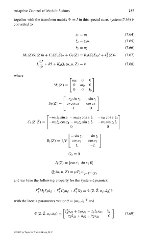
together with the transform matrix = I in this special case, system (7.63) is
converted to

˙ z 1 = u 1 (7.64)
˙ z 2 = z 3 u 1 (7.65)

˙ z 3 = u 2 (7.66)
T
˙
M 3 (Z)S 3 (Z)˙u + C 3 (Z, Z)u + G 3 (Z) = B 3 (Z)K N I + J (Z)λ (7.67)
3
dI
L + RI + K a Q 3 (u, µ, Z) = ν (7.68)
dt
where
 
m 0 0 0
M 3 (Z) =  0 m 0 0 
0 0 I 0
 
−z 2 sin z 1 − sin z 1
S 3 (Z) =  z 2 cos z 1 cos z 1 
1 0
 
−m 0 ˙z 2 sin z 1 − m 0 z 2 cos z 1 ˙z 1 −m 0 cos z 1 ˙z 1
˙
C 3 (Z, Z) =  −m 0 ˙z 2 cos z 1 − m 0 z 2 sin z 1 ˙z 1 −m 0 sin z 1 ˙z 1 
0 0
 
− sin z 1 − sin z 1
B 3 (Z) = 1/P  cos z 1 cos z 1 
L −L
G 3 = 0

J 3 (Z) =[cos z 1 sin z 1 0]

Q 3 (u, µ, Z) = µT 2 u| −1
q=T (Z)
1
and we have the following property for the system dynamics:

T
T
T
S M 3 S 3 ˙u d + S C 3 u d + S G 3 = (Z, Z, u d , ˙u d )θ
˙
3 3 3
T
with the inertia parameters vector θ =[m 0 , I 0 ] and
2

z ˙u d1 + z 2 ˙u d2 + z 2 ˙z 2 u d1 ˙ u d1
2
˙
(Z, Z, u d , ˙u d ) = (7.69)
z 2 ˙u d1 +˙u d2 +˙z 2 u d1 0
© 2006 by Taylor & Francis Group, LLC

FRANKL: “dk6033_c007” — 2006/3/31 — 16:43 — page 287 — #21