Page 368 - Autonomous Mobile Robots

358 Autonomous Mobile Robots

80
60
40
20

0
– 20
– 40
– 60
– 80
– 50 0 50 100 150
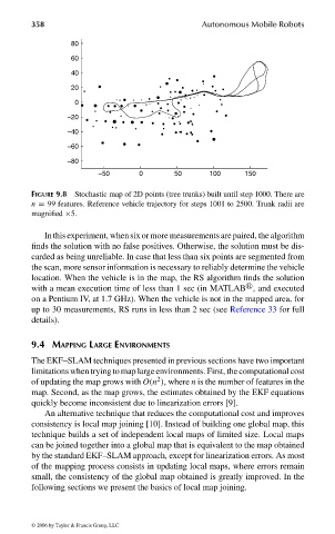
FIGURE 9.8 Stochastic map of 2D points (tree trunks) built until step 1000. There are
n = 99 features. Reference vehicle trajectory for steps 1001 to 2500. Trunk radii are
magnified ×5.

Inthisexperiment, whensixormoremeasurementsarepaired, thealgorithm
finds the solution with no false positives. Otherwise, the solution must be dis-
carded as being unreliable. In case that less than six points are segmented from
the scan, more sensor information is necessary to reliably determine the vehicle
location. When the vehicle is in the map, the RS algorithm finds the solution

with a mean execution time of less than 1 sec (in MATLAB , and executed
on a Pentium IV, at 1.7 GHz). When the vehicle is not in the mapped area, for
up to 30 measurements, RS runs in less than 2 sec (see Reference 33 for full
details).

9.4 MAPPING LARGE ENVIRONMENTS
The EKF–SLAM techniques presented in previous sections have two important
limitations when trying to map large environments. First, the computational cost
2
of updating the map grows with O(n ), where n is the number of features in the
map. Second, as the map grows, the estimates obtained by the EKF equations
quickly become inconsistent due to linearization errors [9].
An alternative technique that reduces the computational cost and improves
consistency is local map joining [10]. Instead of building one global map, this
technique builds a set of independent local maps of limited size. Local maps
can be joined together into a global map that is equivalent to the map obtained
by the standard EKF–SLAM approach, except for linearization errors. As most
of the mapping process consists in updating local maps, where errors remain
small, the consistency of the global map obtained is greatly improved. In the
following sections we present the basics of local map joining.

© 2006 by Taylor & Francis Group, LLC

FRANKL: “dk6033_c009” — 2006/3/31 — 16:43 — page 358 — #28