Page 367 - Autonomous Mobile Robots

Map Building and SLAM Algorithms 357

80
70
60
50
40
30
20
10
0
– 80 – 60 – 40 – 20 0 20 40 60 80
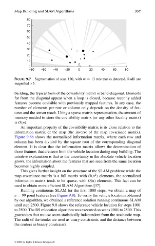
FIGURE 9.7 Segmentation of scan 120, with m = 13 tree trunks detected. Radii are
magnified ×5.

building, the typical form of the covisibility matrix is band-diagonal. Elements
far from the diagonal appear when a loop is closed, because recently added
features become covisible with previously mapped features. In any case, the
number of elements per row or column only depends on the density of fea-
tures and the sensor reach. Using a sparse matrix representation, the amount of
memory needed to store the covisibility matrix (or any other locality matrix)
is O(n).
An important property of the covisibility matrix is its close relation to the
information matrix of the map (the inverse of the map covariance matrix).
Figure 9.6b shows the normalized information matrix, where each row and
column has been divided by the square root of the corresponding diagonal
element. It is clear that the information matrix allows the determination of
those features that are seen from the vehicle location during map building. The
intuitive explanation is that as the uncertainty in the absolute vehicle location
grows, the information about the features that are seen from the same location
becomes highly coupled.
This gives further insight on the structure of the SLAM problem: while the
2
map covariance matrix is a full matrix with O(n ) elements, the normalized
information matrix tends to be sparse, with O(n) elements. This fact can be
used to obtain more efficient SLAM Algorithms [37].
Running continuous SLAM for the first 1000 steps, we obtain a map of
n = 99 point features (see Figure 9.8). To verify the vehicle locations obtained
by our algorithm, we obtained a reference solution running continuous SLAM
until step 2500. Figure 9.8 shows the reference vehicle location for steps 1001
to 2500. The RS relocation algorithm was executed on scans 1001 to 2500. This
guarantees that we use scans statistically independent from the stochastic map.
The radii of the trunks are used as unary constraints, and the distance between
the centers as binary constraints.

© 2006 by Taylor & Francis Group, LLC

FRANKL: “dk6033_c009” — 2006/3/31 — 16:43 — page 357 — #27