Page 138 - Basics of MATLAB and Beyond

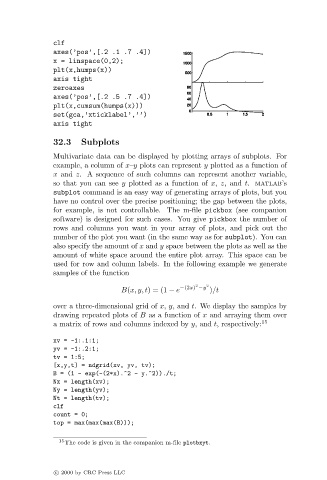
clf
axes(’pos’,[.2 .1 .7 .4])
x = linspace(0,2);
plt(x,humps(x))
axis tight
zeroaxes
axes(’pos’,[.2 .5 .7 .4])
plt(x,cumsum(humps(x)))
set(gca,’xticklabel’,’’)
axis tight

32.3 Subplots
Multivariate data can be displayed by plotting arrays of subplots. For
example, a column of x–y plots can represent y plotted as a function of
x and z. A sequence of such columns can represent another variable,
so that you can see y plotted as a function of x, z, and t. matlab’s
subplot command is an easy way of generating arrays of plots, but you
have no control over the precise positioning; the gap between the plots,
for example, is not controllable. The m-file pickbox (see companion
software) is designed for such cases. You give pickbox the number of
rows and columns you want in your array of plots, and pick out the
number of the plot you want (in the same way as for subplot). You can
also specify the amount of x and y space between the plots as well as the
amount of white space around the entire plot array. This space can be
used for row and column labels. In the following example we generate
samples of the function
2
B(x, y, t)=(1 − e −(2x) −y 2 )/t
over a three-dimensional grid of x, y, and t. We display the samples by
drawing repeated plots of B as a function of x and arraying them over
a matrix of rows and columns indexed by y, and t, respectively: 15

xv = -1:.1:1;
yv = -1:.2:1;
tv = 1:5;
[x,y,t] = ndgrid(xv, yv, tv);
B = (1 - exp(-(2*x).^2 - y.^2))./t;
Nx = length(xv);
Ny = length(yv);
Nt = length(tv);
clf
count = 0;
top = max(max(max(B)));

15 The code is given in the companion m-file plotbxyt.

c 2000 by CRC Press LLC