Page 47 - Basics of MATLAB and Beyond

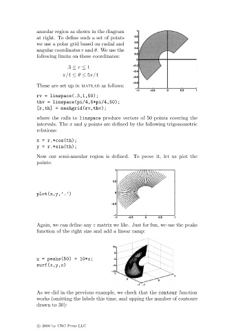
annular region as shown in the diagram
at right. To define such a set of points
we use a polar grid based on radial and
angular coordinates r and θ. We use the
following limits on these coordinates:
.3 ≤ r ≤ 1
π/4 ≤ θ ≤ 5π/4

These are set up in matlab as follows:
rv = linspace(.3,1,50);
thv = linspace(pi/4,5*pi/4,50);
[r,th] = meshgrid(rv,thv);
where the calls to linspace produce vectors of 50 points covering the
intervals. The x and y points are defined by the following trigonometric
relations:
x = r.*cos(th);
y = r.*sin(th);
Now our semi-annular region is defined. To prove it, let us plot the
points:

plot(x,y,’.’)

Again, we can define any z matrix we like. Just for fun, we use the peaks
function of the right size and add a linear ramp:

z = peaks(50) + 10*x;
surf(x,y,z)

As we did in the previous example, we check that the contour function
works (omitting the labels this time, and upping the number of contours
drawn to 30):

c 2000 by CRC Press LLC