Page 150 - Big Data Analytics for Intelligent Healthcare Management

5.8 RESULTS, INTERPRETATION AND DISCUSSION 143

3. Bubbles (O)—Average of all subjects.
4. + individual subject plot.

The baseline data for the EMGav, EMGv, and EMGa was more toward the average of frequency and
duration with a few exceptions for the subjects where the data lay in the high duration and high fre-
quency zone. Initially in all the groups, the subjects or their averages were in the zone of high occur-
rence of TTH for higher durations.
The baseline data for EMGav was mostly in the high duration and high frequency zone, showing
that the subject group consisted of individuals suffering from the most frequently occurring severe pain.
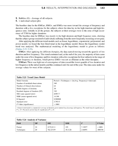
After applying the different trend models such as linear, logarithmic, exponential, polynomial, and
power model, we found the best fitted trend in the logarithmic model. Hence the logarithmic model
trend was analyzed. The mathematical modeling of the logarithmic model is given as follows:
(Tables 5.23–5.25).
EMGv: After applying the different therapies, the data started moving toward the quartile of low
duration and low frequency. This trend continued and, at the end of the year, the majority of data came
under the zone of low frequency and low duration with a few exceptions for four subjects in the range of
higher frequency or duration, which proves EMGv was not as efficient as the other therapies.
EMGav: There was high rate of convergence of data toward the lower quartile of low duration and
low frequency in the initial months and this continued until the end of the year. The data came under the
average values for most of the subjects.

Table 5.23 Trend Lines Model
Model formula Period Techniques (ln(Avg. Frequency)+intercept)
Number of modeled observations 349
Number of filtered observations 61
Model degrees of freedom 30
Residual degrees of freedom (DF) 319
SSE (sum squared error) 4589.77
MSE (mean squared error) 14.388
R-Squared 0.500008
Standard error 3.79315
P-Value (significance) <.0001
A linear trend model is computed for average of duration given natural log of average of frequency. The model may be significant at
P .05. The factor period may be significant at P .05.

Table 5.24 Analysis of Variance
F
Field DF SSE MSE P-Value
Period 24 2472.0111 103 7.15877 <.0001
Techniques 20 762.25159 38.1126 2.64891 .000196