Page 43 - Biomedical Engineering and Design Handbook Volume 1, Fundamentals

20 BIOMEDICAL SYSTEMS ANALYSIS

Outputs

Output layer

Weights
Hidden layer

Input layer

Bias
Inputs
Neural network
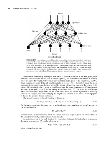
FIGURE 1.10 A neural network model consists of several input layer neurons (nodes), one or more
neurons in the output layer, and one or more layers of hidden layer neurons each consisting of sever-
al neurons. Each neuron in the input layer corresponds to an input parameter, and each neuron in the
output layer corresponds to an output parameter. Each neuron in a layer is connected to each of the
neurons in the next level. In this example only one hidden layer is used. Each of the input neurons is
connected with each neuron in the hidden layer and each neuron in the hidden layer is connected to
each neuron in the output layer. The connection strengths are represented by weights.

There are several training techniques and the most popular technique is the back propagation
technique. Let us assume that for a set of sample inputs X , we know the actual outputs d Initially,
k i.
we do not know the weights, but we could have a random initial guess of the weights w , and W .
j,k i,j
As an example, we could define all weights initially to be w j,k , = W i,j = 0.2 or 0.5. Using the above
equations along with the sample input vector X , we can calculate the output of the system Y . Of
k i
course, this calculated value is going to be different from the actual output (vector if there is more
than one output node) value d , corresponding to the input vector X . The error is the difference
i k
between the calculated output value and the actual value. There are various algorithms to iteratively
calculate the weights, each time changing the weights as a function of the error. The most popular
of these is the gradient descent technique.
The sum of the error in the mth iteration is defined as
m
m
m
m
m
e = d − y = d − F(ΣW H ) = d − F(ΣW f(Σw X ) (1.55)
i i i i i,j j i i,j j,k k
The instantaneous summed squared error at an iteration m, corresponding to the sample data set n,
can be calculated as
m m 2
E = (1/2) Σ(e ) (1.56)
n i
The total error E at each iteration, for all the sample data pairs (input-output), can be calculated as
the sum of the errors E for the individual sample data.
n
Adjusting the weights for each iteration for connections between the hidden layer neurons and
the output layer neurons W can be calculated as
i,j
m
m
W m+1 = W − η(δ E /δW ) (1.57)
i,j i,j i,j
where η is the learning rate.