Page 40 - Biomedical Engineering and Design Handbook Volume 1, Fundamentals

MODELING OF BIOMEDICAL SYSTEMS 17

In developing the above equation, it is assumed that the effect of a memory cell also decays expo-
nentially over a period of time. Thus the production rate of blood lymphocytes at time (t) due to sec-
ondary response (dL /dt) second is due to the sum of the residual effects of all the memory cells formed
B
between 0 and time t − φ , where φ is the time lag between memory cell formation and the appear-
2
2
ance of the secondary response.
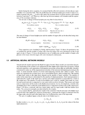
The net rate in change of blood lymphocytes may then be described as
dL /dt = k ∫ t − Φ 1 L (τ)e −K1(t − Φ − τ) dτ+ k ∫ t − Φ 2L (τ)g(τ)e −K4(t − Φ − τ) g(t − Φ )dτ
2
1
B 2 0 T 3 0 T 3
Due to primary response Due to secondary response
+ K L − K L − K L − K L g (1.47)
5 T 6 B 7 B 8 B
Recirculation Death in the blood Migration into tissue due to
target cell presence
The rates of change of tissue lymphocytes and the number of target cells can be described using simi-
lar mass balance
dL /dt = K L g − K L + K L − K L g (1.48)
T 8 B 5 T 6 B 9 T
Increased migration Recirculation Loss due to target cell destruction
dg/dt = (dg/dt) − k L g (1.49)
input 10 T
These equations were simulated by Reddy and Krouskop. Figure 1.8 shows the production rate
of lymphocytes and the number of target cells when the target cells were introduced on day 0 and
again on day 4. Figure 1.9 shows the production rate of lymphocytes and the number of target cells
present in the tissue when the target cells were introduced continuously.

1.5 ARTIFICIAL NEURAL NETWORK MODELS

Neural network models represent the black box type of model. These models are used where the pre-
cise functioning of the system is not understood but the sample input-output data are known. Neural
networks represent a new generation of information processing systems that are artificially (virtually)
constructed to make use of the organizational structure of the neuronal information processing in the
brain. A neural network consists of several interconnecting neurons also called as nodes. These
nodes are organized into an input layer, one or more hidden layers, and an output layer. The number
of input layer nodes in the input layer depends on the number of input variables. The number of
nodes in the output layer is determined by the number of output parameters. Each input parameter is
represented by a node in the input layer, and the each output parameter is represented by a node in
the output layer. The number of nodes in the hidden layer could be variable. Each node in a feed-
forward neural network is connected to every node in the next level of nodes. That means each input
node is connected to all the nodes in the hidden layer neurons. Let us, for simplicity, consider only
one hidden layer. Now, each node in the hidden layer is connected to all the nodes in the output layer.
Figure 1.10 shows a network with four output nodes and five input nodes with four hidden layer
nodes. The connection strengths are determined by the weights.
Let us assume that W represents the weight of the connection from the jth node in the hidden layer
i,j
to the ith node in the output layer, and let us assume that w represents the weight of connection from the
j,k
kth input node to the jth node in the hidden layer. Let X represent the value of kth input node.
k
The sum of weighted inputs to the jth node in the hidden layer is
I =Σw X (1.50)
j j,k k
In other words, I = w X + w X + w X + w X , where X , X , X , X are the values of the four
4
3
1
2
1
1,2 2
1,1 1
1,4 4
1,3 3
input parameters.