Page 93 - Biosystems Engineering

74 Chapter Two

Bode diagram
80
60
Magnitude (dB) 40 0
20

–20
–40
–60
–45

–90
Phase (deg) –135

–180
10 –3 10 –2 10 –1 10 0 10 1 10 2
Frequency (rad/sec)

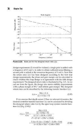
FIGURE 2.21 Bode plot for the designed return ratio L(s).

design requirement (2) would be violated, a single pole is added with
a frequency of 0.5 rad/s. In order to obtain sufficient noise filtering, a
second pole is added at the crossover frequency of 5 rad/s. Now that
the return ratio L(s) has been designed according to the first four
design requirements, the phase and gain margin can be calculated to
check whether this loop design is in agreement with the fifth design
requirement. The designed return ratio is illustrated in Fig. 2.21. As we
can see from the figure, the design also meets stability requirements
with a phase margin of 49.1° and infinite gain margin. The designed
return ratio can be described by the following transfer function L(s):
1
Ls() = 36 s ( + 0 . ) (2.95)
. )(
ss + 05 s + 5 )
(
If we assume that depth sensor H has no relevant dynamics, the
desired controller transfer function C(s) can be calculated by dividing
the designed return ratio L(s) by the open-loop system transfer func-
tion G(s) [Eq. (2.95)]:
36 s ( + 0 1
. )
Ls () ss ( + 05 s + 5 )
. )(
Cs () = =
2
Gs () 11 .7 s + 330 9. s + 3315
s + 15 1s + 139s + 1560s
3
4
2
.
31.(s + 01)(s + 13 . )(s + 1 .69 s + 116 )
2
4
.
(
= (2.96)
2
.
s
(s + 05 )(s + 264s + 283)
. )(s + 5