Page 110 - Cam Design Handbook

THB4 8/15/03 1:01 PM Page 98

98 CAM DESIGN HANDBOOK

Curve (1)
Curve (3)
Curve (2)
Curve (2)
Curve (3) y''
y' Curve (1)

Cam angle q

Cam angle q
(a) Velocity. (b) Acceleration.

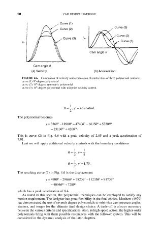
FIGURE 4.6. Comparison of velocity and acceleration characteristics of three polynomial motions:
th
curve (1) 9 -degree polynomial
th
curve (2) 11 -degree symmetric polynomial
th
curve (3) 11 -degree polynomial with midpoint velocity control.

1
q = , y ¢ = no control.
2
The polynomial becomes

y = 336q 5 -18904740q 7 - 6615q 8 + 5320q 9
+
q
6
- 2310420q .
q
+
1011
This is curve (2) in Fig. 4.6 with a peak velocity of 2.05 and a peak acceleration of
7.91.
Last we will apply additional velocity controls with the boundary conditions
1 1
q = , y =
2 2
1
q = , y ¢ =175. .
2
The resulting curve (3) in Fig. 4.6 is the displacement
q
y = 4902968q 6 + 7820q 7 -11235q 8 + 9170q 9
5
-
+ 728q
- 4004q 1011
which has a peak acceleration of 8.4.
As noted in this section, the polynomial techniques can be employed to satisfy any
motion requirement. The designer has great flexibility in the final choice. Matthew (1979)
has demonstrated the use of seventh-degree polynomials to minimize cam pressure angles,
stresses, and torque for the ultimate final design choice. A trade-off is always necessary
between the various criteria and specifications. Also, in high-speed action, the higher-order
polynomials bring with them possible resonances with the follower system. This will be
considered in the dynamic analysis of the later chapters.