Page 109 - Cam Design Handbook

THB4 8/15/03 1:01 PM Page 97

POLYNOMIAL AND FOURIER SERIES CAM CURVES 97

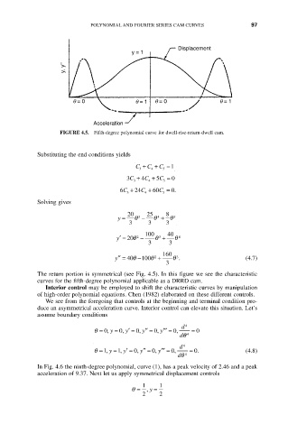
Displacement
y = 1
y, y''

q = 0 q = 1 q = 0 q = 1

Acceleration
FIGURE 4.5. Fifth-degree polynomial curve for dwell-rise-return-dwell cam.

Substituting the end conditions yields

C + C + C = 1
3 4 5
3C + 4C + 5C = 0
3 4 5
6C + 24C + 60C = 0.
3 4 5
Solving gives

20 25 8
y = q 3 - q 4 + q 5
3 3 3
100 40
y ¢ = 20q 2 - q 3 + q 4
3 3
160
q
-
3
y ¢¢ = 40100q 2 + q . (4.7)
3
The return portion is symmetrical (see Fig. 4.5). In this figure we see the characteristic
curves for the fifth-degree polynomial applicable as a DRRD cam.
Interior control may be employed to shift the characteristic curves by manipulation
of high-order polynomial equations. Chen (1982) elaborated on these different controls.
We see from the foregoing that controls at the beginning and terminal condition pro-
duce an asymmetrical acceleration curve. Interior control can elevate this situation. Let’s
assume boundary conditions
d 4
q = 0, y = 0, y ¢ = 0, y ¢¢ = 0, y ¢¢¢ = 0, = 0
d q 4
d 4
q =1, y =1, y ¢ = 0, y ¢¢ = 0, y ¢¢¢ = 0, = 0. (4.8)
d q 4
In Fig. 4.6 the ninth-degree polynomial, curve (1), has a peak velocity of 2.46 and a peak
acceleration of 9.37. Next let us apply symmetrical displacement controls

1 1
q = , y =
2 2