Page 121 - Cam Design Handbook

THB5 8/15/03 1:52 PM Page 109

CAM MOTION SYNTHESIS USING SPLINE FUNCTIONS 109

The use of polynomial functions is probably the most general scheme for interpolat-
ing a set of discrete constraints. In its basic form, the functions are applied by using a
polynomial equation of a degree that is one less than the number of constraints to be sat-
isfied. One of the polynomial coefficients can be established for each constraint that must
be satisfied. If the number of constraints is sizable, then the polynomial will be of high
degree. High-degree polynomials often display some undesirable characteristics between
constraints. Sometimes the polynomial coefficients become computationally difficult to
determine because of the large systems of ill-conditioned equations that may occur
(Forsythe et al., 1977). The polynomial approach can be extended to address nonrigid fol-
lower behavior under certain conditions. The classic polydyne method is an example.
Early in the advent of computer-aided design (CAD) techniques, especially those used
to define curves and surfaces, curve fitting methods were the subject of intense study. Farin
(1988) offers a very readable treatment of the broad area of curves and surfaces, includ-
ing several that have potential for cam applications. Of likely interest to cam designers
are Bezier curves and splines. Both are piecewise continuous functions, and in certain cir-
cumstances are equivalent. Both are defined by control points but differ in the effects of
changing these points. A change in a control point for a Bezier curve affects the entire
curve, whereas a similar change in a spline function results in a local influence. Conse-
quently, splines afford the designer greater local control and therefore are more adaptable
when design constraints are defined locally. Such is usually the case with cams when the
designer must satisfy discrete kinematic constraints and preserve continuity locally.
The methods described here employ splines, in particular piecewise continuous poly-
nomials called basis splines (B-splines), to define displacement curves for cams. The basic
approach is described and illustrated by example and then is extended to accommodate
slightly more advanced forms of splines and is applied to nonrigid followers and to the
synthesis of three-dimensional cam surfaces.
Spline functions are well known and well understood, and practical procedures for eval-
uating them have been long known (deBoor, 1972; Cox, 1972). An especially nice char-
acteristic of spline functions for cam motion programs is that a piecewise polynomial
constructed of B-splines can be made to have continuous derivatives up to any order.
However, since continuity in the second derivative is usually adequate for cams, the B-
splines often need only be cubic functions, regardless of the number of constraints present.
There appears to be little practical difficulty in using splines of order five or six on a routine
basis, though. (The order of spline functions will be more clearly defined later.) The reduc-
tion in the degree of the functions involved effectively avoids the numerical difficulties
associated with high-degree polynomials mentioned earlier.

5.2 APPLICATION OF NONRATIONAL B-SPLINES
TO MOTION SYNTHESIS

5.2.1 Basic Theory

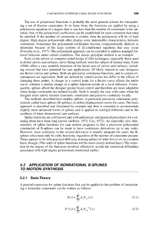
A general expression for spline functions that can be applied to the problem of interpolat-
ing n kinematic constraints can be written as follows:
n
Sx () = Â A N () (5.1)
x
j j k ,
j=1
n
S () = Â A N j k , 1 () x () (5.2)
1 ()
x
j
j 1
=