Page 123 - Cam Design Handbook

THB5 8/15/03 1:52 PM Page 111

CAM MOTION SYNTHESIS USING SPLINE FUNCTIONS 111

As indicated in item 2, if the F j is a velocity constraint, then the E i,j in the equation con-
taining the F j will be first derivatives. If the F j is an acceleration, then the E i,j will be second
derivatives, and so on. Written in matrix notation the system of equations above becomes
[][ F (5.6)
EA] = [].
4. Solve the system of equations above for the coefficients A j .
5. Using the methods below, evaluate the B-splines or B-spline derivatives as needed
to determine displacement, velocity, acceleration, jerk, and other elements between
constraints.

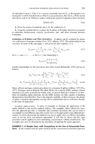
Evaluation of B-Splines and Their Derivatives. B-splines can be evaluated by means
of a well-known recurrence relation (Cox, 1972; deBoor, 1972). This relationship for the
case here, in terms of the cam angle, x, and given the knot sequence, T, is
xT T - x
-
+
x
N () = j N x ()+ jk N x () (5.7)
jk , jk , -1 j+1 k , -1
T - T T - T
+-1
jk j jk j+1
+
for k > 1 and j = 1,... , n. For k = 1, the relationship is
x
T , 1 Ï j £< T j 1
+
x
N () = Ì (5.8)
j,1
Ó , 0 otherwise.
Similar relationships for the derivatives have been found (Butterfield, 1976) and are as
follows:
È N jk , -1 ( m- ) 1 x () N j+1 k , -1 ( m- ) 1 x ()˘
()
m
N jk , x () = ( k - ) 1 Í - ˙ (5.9)
Î T jk - T j T jk - T j+1 ˚
+
+-1
xT
k -1
+
m
m
m
N jk , () x () = Ê Ë km -1 ˆ ¯ È Í Î T jk - - j T j N jk , -1 () x ()+ T T jk jk - - T x j+1 N j+1 k , -1 () () ˘ ˙ ˚ (5.10)
x .
-
+
+-1
Many software packages contain procedures for evaluating B-splines (deBoor, 1977; Foy,
1977). Packages such as MatLab (The Math Works, Inc.) and the IMSL software (Visual
Numerics) are easily accessed and widely used. At present MatLab is limited in its flexi-
bility for handling spline functions, but the IMSL routines are fully capable of handling
the procedures described here. Due to the general availability of these resources, the details
of spline evaluation and equation solving will be omitted here and we will move directly
to the issue of application.
example applications: A series of examples to illustrate the application of the
spline method to cam motion synthesis follows. The examples, taken collectively, show
how the approach provides a consistent and systematic procedure that can be used to
accomplish several different aims that usually have to be approached using different pro-
cedures. It will be shown that the method is as easy to apply and is as effective in routine
cases as are the more conventional approaches. It will also be shown that the same
procedure can be applied in more demanding circumstances without modification. The
examples also serve to demonstrate the mechanics of applying the spline approach.
EXAMPLE 1: A Simple Case, with Comparison to the Use of Polynomial Func-
tions In this example both the spline method and the conventional polynomial approach