Page 122 - Cam Design Handbook

THB5 8/15/03 1:52 PM Page 110

110 CAM DESIGN HANDBOOK

n
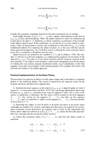
S () = Â A N 2 () x () (5.3)
2 ()
x
j j k ,
=
j 1
. .
. .
. .
n
S () = Â A N j k , () x () (5.4)
m
m
()
x
j
j=1
Usually, the equations containing derivatives beyond acceleration are not needed.
Each spline function, N j,k (x), j = 1,..., n, has a unique representation on the interval
[x min, x max] (Curry and Schoenburg, 1966). The spline function of order k is continuous up
to derivatives of order k - 2. Therefore, to obtain continuous acceleration, at least fourth-
order splines must be used. If the coefficients, A j, are known it is an easy matter to inter-
polate values of displacement, velocity, and acceleration on the interval [x min, x max] using
established methods for evaluating the spline functions. As is the case with the conven-
tional polynomial approach, one coefficient can be evaluated for each constraint that is
given. For n constraints, n B-splines must be used.
Spline functions are defined by the variables k, T, n, and A j (deBoor, 1978). The vari-
able, T, referred to as the knot sequence, is a nondecreasing sequence of real points on the
interval [x min, x max]. The order, k, of the spline functions and the selection of points in the
knot sequence, T, are subject to the designer’s control and consequently provide the means
of refining the cam motion program mentioned earlier. Local adjustments in the knot
sequence will cause local changes in the motion program. The examples that follow will
illustrate this feature of the spline approach.
Practical Implementation of the Basic Theory
The procedure for applying B-splines is really rather simple and is described in a stepwise
fashion in the following outline. The means of determining the required values for the
B-spline functions and derivatives appears later.
1. Establish the knot sequence on the interval [x min, x max]. A single B-spline of order k
requires k + 1 consecutive knots (de Boor, 1972). For cam design applications, there must
be knots as x min and at x max and these knots must be repeated k times. For a series of B-
splines to interpolate n constraints, the first spline will be located on the knot sequence
T 1 ,..., T k+1 , the second on the sequence T 2 ,..., T k+2 , the third on the sequence
th
T 3,..., T k+3, and so on until the n spline on the sequence T n,... , T k+n. The total number
of knots then is k + n.
2. Determine the values of each B-spline or B-spline derivative at all points where
constraints are defined. For velocity constraints first derivatives are required; for acceler-
ation constraints second derivatives are required, and so forth. In the expressions that
follow, these values are referred to as Ei,j, (i, j = 1,... , n), where the first subscript iden-
tifies the constraint and the second the spline function.
3. Collect the constraint values, F j (j = 1,..., n), and form the linear system of
equations
AE , + AE , +L + A E 1, n = F 1
n
11 2
11 1
M M M M
AE + A E +L + A E = F . (5.5)
1 n 1 , 2 n 2 , n n n , n