Page 434 - Cam Design Handbook

THB13 9/19/03 7:56 PM Page 422

422 CAM DESIGN HANDBOOK

Ê 0 1 0 0 0 ˆ Ê ˆ 0
Á -r 0 -r 1 r 0 00 ˜ Á ˜ 0
Á ˜ Á ˜
˙ x = Á 00 0 10 x + Á ˜ 0 u (13.46)
˜
Á 0 0 0 0 1 ˜ Á ˜
0
Á ˜ Á ˜
Ë 0 0 0 0 ¯ 0 Ë ¯ 1
and
0 Ê ˆ 1 Ê ˆ
0 Á ˜ 0 Á ˜
Á ˜ Á ˜
1
0
x 0 () = Á ˜ , x 1 () = Á ˜ . (13.47)
Á ˜ Á ˜
0
0
Á ˜ Á ˜
0 Ë ¯ 0 Ë ¯
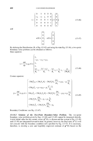
By defining the Hamiltonian, H, of Eq. (13.42) and using the state Eq. (13.46), a two-point
boundary-value problem can be obtained as follows:
State equation:
Ê ˆ
Á x 2 ˜
Á -rx - r x + rx ˜
0 3
1 2
0 1
Á ˜
∂H x
˙ x = ( xp t Á 4 ˜
,, ) =
∂ p Á x ˜
Á 5 ˜
Á rr (r 1 2 - ) rr r 0 p 5 ˜ (13.48)
r
0
01
01
Á K x 1 + K x 2 - K x 3 + K x 4 - 2 WK 2 ˜
Ë k k k k 2 k ¯
Costate equation:
Ê ˙˙ 2 2 ∂N F rr ˆ
01
2
2
2
Á - WF r + W F N F - W F N F ∂x + pr - p K ˜
3
205
3
fe
fe
1
fe 0
Á 1 k ˜
Á ˙˙ r 1 2 - r 0 ˜
2
Á - Wr F fe - p 1 + p r - p 5 K ˜
2 1
11
Á k ˜
∂H Á ∂ N rr ˜
˙˙
˙ p = ( xp t Wr F - W K F N 2 - W F N F - pr + p 01
,, ) = 2
2
2
2
fe
∂ x Á 103 k fe F 3 fe fe F ∂ x 305 K ˜ (13.49)
Á 3 k ˜
Á 2 ∂ N F r 0 ˜
Á - 2 WF N F ∂ x - p - p 5 K ˜
3
3
fe
Á 4 k ˜
Á ∂ N ˜
˙˙
2
Á - 2 WK F - 2 W F N F - p ˜
Ë 1 k fe 3 fe F ∂ x 4 ¯
5
Boundary Conditions: use Eq. (13.47).
13.5.8.2 Solution of the Two-Point Boundary-Value Problem. The two-point
boundary-value problem given by Eqs. (13.48) and (13.49) cannot be integrated directly.
(0)
A trial initial value for the costate vector, p (0), is chosen and the system of Eq. (13.48)
(0)
and (13.49) are integrated forward in time. In general, however, the final state, x (1) will
not coincide with the boundary condition x(1) specified by Eq. (13.47). It is necessary,
(0)
therefore, to develop a new and hopefully improved estimate of p (0) based on the