Page 435 - Cam Design Handbook

THB13 9/19/03 7:56 PM Page 423

CAM SYSTEM DYNAMICS—RESPONSE 423

(0)
difference between x (1) and x(1). The iteration formula relating the correction term for
the previous initial costate to the new costate is:
-1
x())
p ( j+ ) 1 () =0 p () -{ P p ()( j () 0 1 )} ( x () - 1 (13.50)
1
,
j ()
j ()
0
x
(j)
where P x(p (0),1) is the influence function matrix and is given by
Ê ∂ x () 1 ◊◊◊ ∂ x () ˆ
1
1
1
Á ∂ p () 0 ∂ p ()˜
0
Á 1 . 5 . ˜
Á ˜ ∂ x() 1
Pp ()( j () 01 ) = Á . . ˜ = . (13.51)
,
x
Á ˜ ∂ p() 0
Á . . ˜
Á ∂ x () 1 ∂ x () ˜
1
5
5
Á ◊◊◊ ˜
0
Ë ∂ p () 0 ∂ p ()¯
1
5
Since the explicit relationship between the vectors p(0) and x(1) is not known, the influ-
ence function matrix, P x , cannot be easily calculated. One approach involves the pertur-
bations of each of the components p k (0), k = 1,..., 5 of the costate vector p(0) and the
approximation
∂x 1 () D x 1 ()
ª k = , 5. (13.52)
1 ◊◊◊,
∂ () D p 0 ()
p
0
k k
Such a differencing procedure faces the problem of choosing the magnitude of the per-
turbations. Large perturbations may cause the difference approximation to be inaccurate,
while small perturbations introduce numerical inaccuracies associated with integration,
roundoff, and truncation errors.
Another approach is to take partial derivatives of Eqs. (13.48) and (13.49) with respect
to the initial value of the costate vector, p(0), and interchange the order of differentiation
(since continuity with respect to p(0) and t is assumed). The resulting two-point boundary-
value problem is derived in App. F, with each subsequent new approximation for
the vector, p (j+1) (0) given by the iteration formula of Eq. (13.50). This approach to the solu-
tion of the two-point boundary-value problem is called the Variation of Extremals, also
known as the Generalized Newton-Raphson algorithm. It is a second-order gradient tech-
(0)
nique and hence, a good initial approximation for the costate vector, p (0), is usually
needed for convergence.
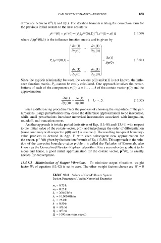
13.5.8.3 Minimization of Output Vibrations. To minimize output vibrations, weight
factor W 3 of equation (13.42) is set to zero. The other weight factors chosen are W 1 = 0
TABLE 13.3 Values of Cam-Follower System
Design Parameters Used in Numerical Examples
m o = 0.75lb
m f = 0.25lb
k s = 200.0lb/in
k f = 10,000.0lb/in
s p = 75.0lb
h = 0.50in
q 1 = p/3rad
q 2 = p/3rad
W= 1000rpm (cam speed)