Page 135 - Chemical engineering design

115
FUNDAMENTALS OF ENERGY BALANCES
Significance of the pinch
The pinch divides the system into two distinct thermodynamic regions. The region above
the pinch can be considered a heat sink, with heat flowing into it, from the hot utility,
but not out of it. Below the pinch the converse is true. Heat flows out of the region to
the cold utility. No heat flows across the pinch.
If a network is designed that requires heat to flow across the pinch, then the consumption
of the hot and cold utilities will be greater than the minimum values that could be achieved.

3.17.2. The problem table method
The problem table is the name given by Linnhoff and Flower to a numerical method for
determining the pinch temperatures and the minimum utility requirements; Linnhoff and
Flower (1978). Once understood, it is the preferred method, avoiding the need to draw the
composite curves and manoeuvre the composite cooling curve using, for example, tracing
paper or cut-outs, to give the chosen minimum temperature difference on the diagram.
Theprocedure isasfollows:
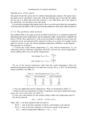
1. Convert the actual stream temperatures T act into interval temperatures T int by
subtracting half the minimum temperature difference from the hot stream temperatures,
and by adding half to the cold stream temperatures:
T min
hot streams T int D T act
2
T min
cold streams T int D T act C
2
The use of the interval temperature rather than the actual temperatures allows the
Ž
minimum temperature difference to be taken into account. T min D 10 C for the problem
being considered; see Table 3.4.

Table 3.4. Interval temperatures for T min D 10 ° C
Stream Actual temperature Interval temperature
1 180 60 175 55
2 150 30 145 25
3 20 135 (25) 140
4 80 140 85 (145)

2. Note any duplicated interval temperatures. These are bracketed in Table 3.4.
3. Rank the interval temperatures in order of magnitude, showing the duplicated temper-
atures only once in the order; see Table 3.5.
4. Carry out a heat balance for the streams falling within each temperature interval:
For the nth interval:
H n D CP c CP h T n

where H n D net heat required in the nth interval
CP c D sum of the heat capacities of all the cold streams in the interval
CP h D sum of the heat capacities of all the hot streams in the interval
T n D interval temperature difference D T n 1 T n