Page 270 - Chiral Separation Techniques

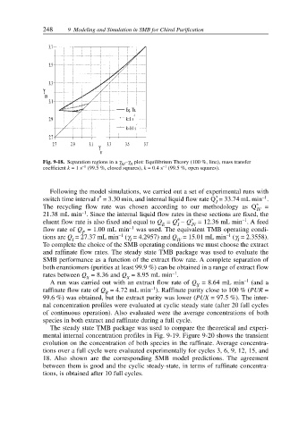
248 9 Modeling and Simulation in SMB for Chiral Purification

Fig. 9-18. Separation regions in a γ –γ plot: Equilibrium Theory (100 %, line), mass transfer
II
III
–1
–1
coefficient k = 1 s (99.5 %, closed squares), k = 0.4 s (99.5 %, open squares).
Following the model simulations, we carried out a set of experimental runs with
–1
*
*
switch time interval t = 3.30 min, and internal liquid flow rate Q = 33.74 mL min .
I
The recycling flow rate was chosen according to our methodology as Q * IV =
–1
21.38 mL min . Since the internal liquid flow rates in these sections are fixed, the
*
–1
eluent flow rate is also fixed and equal to Q = Q – Q * IV = 12.36 mL min . A feed
I
E
flow rate of Q = 1.00 mL min –1 was used. The equivalent TMB operating condi-
F
–1
–1
tions are Q = 27.37 mL min (γ = 4.2957) and Q = 15.01 mL min (γ = 2.3558).
I I IV I
To complete the choice of the SMB operating conditions we must choose the extract
and raffinate flow rates. The steady state TMB package was used to evaluate the
SMB performance as a function of the extract flow rate. A complete separation of
both enantiomers (purities at least 99.9 %) can be obtained in a range of extract flow
–1
rates between Q = 8.36 and Q = 8.95 mL min .
X X
A run was carried out with an extract flow rate of Q = 8.64 mL min –1 (and a
X
–1
raffinate flow rate of Q = 4.72 mL min ). Raffinate purity close to 100 % (PUR =
R
99.6 %) was obtained, but the extract purity was lower (PUX = 97.5 %). The inter-
nal concentration profiles were evaluated at cyclic steady state (after 20 full cycles
of continuous operation). Also evaluated were the average concentrations of both
species in both extract and raffinate during a full cycle.
The steady state TMB package was used to compare the theoretical and experi-
mental internal concentration profiles in Fig. 9-19. Figure 9-20 shows the transient
evolution on the concentration of both species in the raffinate. Average concentra-
tions over a full cycle were evaluated experimentally for cycles 3, 6, 9, 12, 15, and
18. Also shown are the corresponding SMB model predictions. The agreement
between them is good and the cyclic steady-state, in terms of raffinate concentra-
tions, is obtained after 10 full cycles.