Page 104 - Circuit Analysis II with MATLAB Applications

Chapter 3 Elementary Signals

vt
3
{
2
2t + 1
1 – t + 3
|
t
0 1 2 3

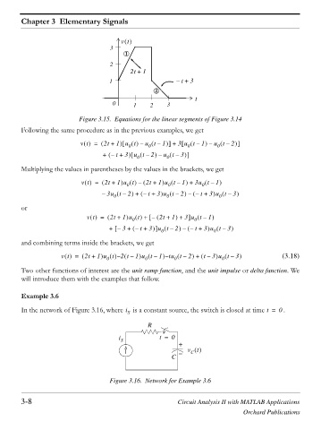
Figure 3.15. Equations for the linear segments of Figure 3.14
Following the same procedure as in the previous examples, we get

vt = 2t + 1 u t –> 0 u t – 1 @ 3u t – 1 – u t – 2 @
+

>
0
0
0
+ – + 3 u t – > 0 2 – u t – 3 @
t

0
Multiplying the values in parentheses by the values in the brackets, we get
vt = 2t + 1 u t – 2t + 1 u t – 1 + 3u t – 1

0
0
0
3u t – – 0 2 + – t + 3 u t – 2 – – t + 3 u t – 3

0
0
or
vt = 2t + 1 u t + – > 2t + 1 + 3 u t – 1

@

0
0
+ – 3 + – t + 3 @ u t – 0 2 – – t + 3 u t – 3

>
0
and combining terms inside the brackets, we get
vt = 2t + 1 u t 2t – – 1 u t – 1 – tu t – 2 + t – 3 u t – 3 (3.18)

0
0
0
0
Two other functions of interest are the unit ramp function, and the unit impulse or delta function. We
will introduce them with the examples that follow.
Example 3.6
In the network of Figure 3.16, where is a constant source, the switch is closed at time t = . 0
i
S
R
i S t = 0
+
v t
C
C
Figure 3.16. Network for Example 3.6
3-8 Circuit Analysis II with MATLAB Applications
Orchard Publications