Page 102 - Circuit Analysis II with MATLAB Applications

Chapter 3 Elementary Signals

vt = v t + v t + v t + v t
4
3
2
1
= Au t –> 0 u t – T @ – A u t – T – u t – 2T @ (3.12)

>

0
0
0
+Au t – > 0 2T – u t – 3T @ – A u t – 3T – u t – 4T @

>

0
0
0
Combining like terms, we get
vt = Au t –> 0 2u t – T + 2u t – 2T – 2u t – 3T + } @ (3.13)

0
0
0
Example 3.3
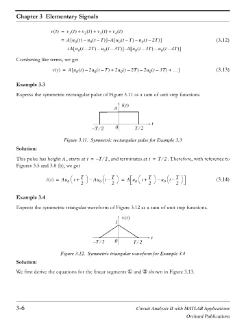
Express the symmetric rectangular pulse of Figure 3.11 as a sum of unit step functions.
it
A
t
– T 2 0 T2
e
e
Figure 3.11. Symmetric rectangular pulse for Example 3.3
Solution:
A
This pulse has height , starts at t = – T 2 , and terminates at t = T 2 . Therefore, with reference to
e
e
Figures 3.5 and 3.8 (b), we get
it = Au 0 § © t + T · --- ¹ – Au 0 § © t – T · --- ¹ = Au 0 § © t + T · --- ¹ – u 0 § © t – T · --- ¹ (3.14)
2
2
2
2
Example 3.4
Express the symmetric triangular waveform of Figure 3.12 as a sum of unit step functions.
vt
1
t
– T2 0 T2
e
e
Figure 3.12. Symmetric triangular waveform for Example 3.4
Solution:
We first derive the equations for the linear segments { and | shown in Figure 3.13.

3-6 Circuit Analysis II with MATLAB Applications

Orchard Publications