Page 101 - Circuit Analysis II with MATLAB Applications

The Unit Step Function

The unit step function offers a convenient method of describing the sudden application of a voltage
or current source. For example, a constant voltage source of 24 V applied at t = 0 , can be denoted
as 24u t V . Likewise, a sinusoidal voltage source v t = V cos ZtV that is applied to a circuit at
0
m
t = t 0 , can be described as vt = V cos Zt u t – t 0 V . Also, if the excitation in a circuit is a rect-

0
m
angular, or triangular, or sawtooth, or any other recurring pulse, it can be represented as a sum (dif-
ference) of unit step functions.
Example 3.2

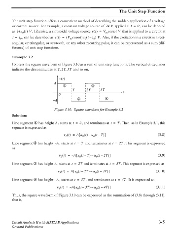
Express the square waveform of Figure 3.10 as a sum of unit step functions. The vertical dotted lines
indicate the discontinuities at T2T3T and so on.

vt
A
{ }
T 2T 3T
0 t
– A | ~

Figure 3.10. Square waveform for Example 3.2
Solution:

A
Line segment { has height , starts at t = 0 , and terminates at t = T . Then, as in Example 3.1, this
segment is expressed as
v t = Au t – u t – T @ (3.8)

>
0
0
1
Line segment | has height A– , starts at t = T and terminates at t = 2T . This segment is expressed
as
v t = – A u t – T – u t – 2T @ (3.9)

>

0
2
0
A
Line segment } has height , starts at t = 2T and terminates at t = 3T . This segment is expressed as
v t = Au t – 2T – u t – 3T @ (3.10)

>

0
0
3
Line segment ~ has height A– , starts at t = 3T , and terminates at t = 4T . It is expressed as
v t = – A u t – 3T – u t – 4T @ (3.11)

>
0
0
4
Thus, the square waveform of Figure 3.10 can be expressed as the summation of (3.8) through (3.11),
that is,
Circuit Analysis II with MATLAB Applications 3-5
Orchard Publications