Page 100 - Circuit Analysis II with MATLAB Applications

Chapter 3 Elementary Signals

v u t – S 0 T
v out

t
0 T

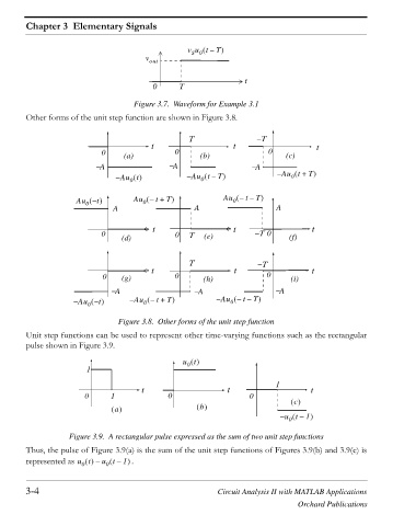
Figure 3.7. Waveform for Example 3.1
Other forms of the unit step function are shown in Figure 3.8.

7 7
t t t
0 (a) 0 (b) 0 (c)

A A A
– Au t – Au t – 0 T – Au t + 0 T
0

t
Au – Au – + 0 t T Au – – 0 t T
0
A A A
t t t
0 (d) 0 7 (e) 7 0 (f)

7 7
t t t
0 (g) 0 (h) 0 (i)

A A A
t
– Au – – Au – + 0 t T – Au – – 0 t T
0
Figure 3.8. Other forms of the unit step function
Unit step functions can be used to represent other time-varying functions such as the rectangular
pulse shown in Figure 3.9.

u t
0
1
1
t t t
0 1 0 0
c
a b
u t – – 0 1

Figure 3.9. A rectangular pulse expressed as the sum of two unit step functions
Thus, the pulse of Figure 3.9(a) is the sum of the unit step functions of Figures 3.9(b) and 3.9(c) is
represented as u t – u t – 1 .

0
0
3-4 Circuit Analysis II with MATLAB Applications

Orchard Publications