Page 97 - Circuit Analysis II with MATLAB Applications

Chapter 3

Elementary Signals

T his chapter begins with a discussion of elementary signals that may be applied to electric net-

works. The unit step, unit ramp, and delta functions are then introduced. The sampling and
sifting properties of the delta function are defined and derived. Several examples for expressing
a variety of waveforms in terms of these elementary signals are provided.

3.1 Signals Described in Math Form

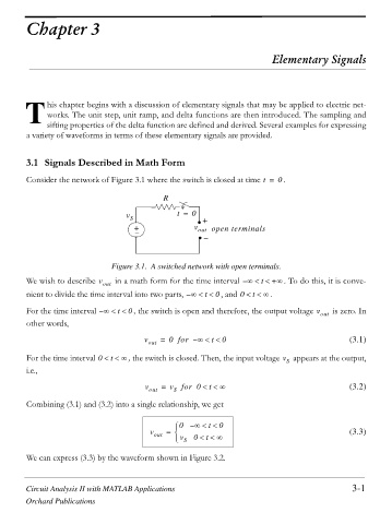
Consider the network of Figure 3.1 where the switch is closed at time t = . 0

R

v S t = 0 +
+ v out open terminals

Figure 3.1. A switched network with open terminals.
–
We wish to describe v out in a math form for the time interval f +f . To do this, it is conve-
t
t
nient to divide the time interval into two parts, f – t 0 , and 0 f .
For the time interval f – t 0 the switch is open and therefore, the output voltage v out is zero. In
other words,

t
v out = 0for – f 0 (3.1)
t
For the time interval 0 f the switch is closed. Then, the input voltage v S appears at the output,
i.e.,

t
v out = v S for 0 f (3.2)
Combining (3.1) and (3.2) into a single relationship, we get

t
–
­ 0 f 0
v out = ® (3.3)
t
S
¯ v 0 f
We can express (3.3) by the waveform shown in Figure 3.2.

Circuit Analysis II with MATLAB Applications 3-1
Orchard Publications