Page 94 - Circuit Analysis II with MATLAB Applications

Chapter 2 Resonance

1
100
1
8
9
2
--------- =
Z = ------- – 100 --------------------------- – ---------- = 10 – 10 = 9 u 10 8
0 LC L 2 10 – 3 u 10 – 6 10 – 6
and thus
8
Z = 9 u 10 = 30 000 r s

e
0
b.
BW = Z e Q = 30 000 50 = 600 r s
e

e
0
c.
–
Z = Z – BW 2 = 30 000 300 = 29 700 r s
e

e

0
1
Z = Z + BW 2 = 30 000 + 300 = 30 300 r s
e

e
0
2
6
4
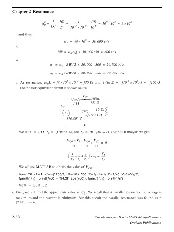
d. At resonance, jZ L = j3 u 10 u 10 – 3 = j30 : and 1jZ Ce = – j10 – 4 u 10 e 3 = – j100 . 3 e
0 0
The phasor equivalent circuit is shown below.
V
C0
`
1 : j30 :
V S
10 :
– j100 3 :
e
170 0q V
‘
We let z = 1 : , z = – j100 3 : , and z = 10 + j30 : . Using nodal analysis we get:
e
1
2
3
V – V V V
C0
C0
S
C0
---------------------- + --------- + --------- = 0
z 1 z 2 z 3
1
1
§ ---- + ---- + ---- V = V S
1 ·
------
© z 1 z 2 z 3 ¹ C0 z 1
We wil use MATLAB to obtain the value of V C0 .
Vs=170; z1=1; z2= j*100/3; z3=10+j*30; Z=1/z1+1/z2+1/z3; Vc0=Vs/Z;...
fprintf(' \n'); fprintf('Vc0 = %6.2f', abs(Vc0)); fprintf(' \n'); fprintf(' \n')
Vc0 = 168.32
6. First, we will find the appropriate value of C 2 . We recall that at parallel resonance the voltage is
maximum and the current is minimum. For this circuit the parallel resonance was found as in
(2.37), that is,
2-28 Circuit Analysis II with MATLAB Applications
Orchard Publications