Page 90 - Circuit Analysis II with MATLAB Applications

Chapter 2 Resonance

2.12 Solutions to Exercises

L
1. At series resonance Z = R = 100 and thus R = 100 : . We find from Q 0S = Z LR where
e
0
0
Z = 2Sf . Also,
0 0
Z Z 2S u 10 6
0
0
Q 0S = ------------------ = --------- = --------------------------------- = 50
Z –
2 Z 1 BW 2S u 20 u 10 3
Then,
RQ 100 u 50
˜
0S
L = ----------------- = --------------------- = 0.796 mH
Z 6
0 2S u 10
2
and from Z = 1LC
e
0
1 1
C = --------- = -------------------------------------------------------------- = 31.8 pF
2
Z L 2S u 10 6 2 u 7.96 u 10 – 4
0
Check with MATLAB:
f0=10^6; w0=2*pi*f0; Z0=100; BW=2*pi*20000; w1=w0-BW/2; w2=w0+BW/2;...
R=Z0; Qos=w0/BW; L=R*Qos/w0; C=1/(w0^2*L); fprintf(' \n');...
fprintf('R = %5.2f Ohms \t', R); fprintf('L = %5.2e H \t', L);...
fprintf('C = %5.2e F \t', C); fprintf(' \n'); fprintf(' \n');
R = 100.00 Ohms L = 7.96e-004 H C = 3.18e-011 F
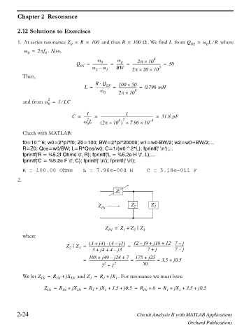
2.

Z 1

Z IN Z 2 Z 3

Z IN = Z + Z __ Z 3
1
2
where
j3
4 –
3 +

j4 ˜
------------------------------------------- ----------
Z __ Z = ------------------------------------------ = 12 – j9 + j16 + 12 7 – j j
˜
2
3
7 –
j
7 +
–
3 +
j4 +
4 j3
168 + j49 – j24 + 7 175 + j25
= ---------------------------------------------- = ----------------------- = 3.5 + j0.5
2
7 + 1 2 50
We let Z IN = R IN + jX IN and Z = R + jX 1 . For resonance we must have
1
1
Z IN = R IN + jX IN = R + jX + 3.5 + j0.5 = R IN + 0 = R + jX + 3.5 + j0.5
1
1
1
1
2-24 Circuit Analysis II with MATLAB Applications
Orchard Publications