Page 88 - Circuit Analysis II with MATLAB Applications

Chapter 2 Resonance

2.11 Exercises

1. A series RLC circuit is resonant at f = 1MHz with Z = 100 : and its half-power bandwidth
0
0
is BW = 20 KHz . Find RL , and for this circuit.
C
,
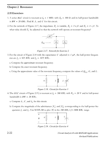
2. For the network of Figure 2.17, the impedance Z 1 is variable, Z = 3 + j4 and Z = 4 – j3 . To
2
3
what value should Z 1 be adjusted so that the network will operate at resonant frequency?

Z 1

Z IN Z 2 Z 3

Figure 2.17. Network for Exercise 2
3. For the circuit of Figure 2.18 with the capacitance adjusted to 1 PF , the half-power frequen-
C
cies are f = 925 KHz and f = 1075 KHz .
2
1
a. Compute the approximate resonant frequency.

b. Compute the exact resonant frequency.
G
c. Using the approximate value of the resonant frequency, compute the values of Q op , , and .
L

`
G L C

Figure 2.18. Circuit for Exercise 3
4. The GLC circuit of Figure 2.19, is resonant at f = 500 KHz with V = 20 V and its half-power
0
0
bandwidth is BW = 20 KHz .
a. Compute , , and for this circuit.
LC
I
0
b. Compute the magnitude of the admittances Y 1 and Y 2 corresponding to the half-power fre-
f
f
quencies and . Use MATLAB to plot Y in the 100 KHz d d 1000 KHz range.
f
1
2
+
V G L ` C

Figure 2.19. Circuit for Exercise 4

2-22 Circuit Analysis II with MATLAB Applications

Orchard Publications