Page 342 - Classification Parameter Estimation & State Estimation An Engg Approach Using MATLAB

TIME-OF-FLIGHT ESTIMATION OF AN ACOUSTIC TONE BURST 331

value of J such that J << N. Hopefully,
n is large for the first few n,and
then drops down rapidly to zero.

The computational structure of the estimator based on a covariance model
A straightforward implementation of (9.20) is not very practical. The
expression must be evaluated for varying values of t. Since the dimen-
sion of C zjt is large, this is not computationally feasible.
The problem will be tackled as follows. First, we define a moving
window for the measurements z n . The window starts at n ¼ i and ends at
n ¼ i þ I 1. Thus, it comprises I samples. We stack these samples into
a vector x(i) with elements x n (i) ¼ z nþi . Each value of i corresponds to a
hypothesized value t ¼ i . Thus, under this hypothesis, the vector x(i)
contains the direct response with t ¼ 0, i.e. x n (i) ¼ a h(n )þ
a r(n ) þ v(n ). Instead of applying operation (9.20) for varying t, t is
fixed to zero and z is replaced by the moving window x(i):

J 1
T 2
X
yðiÞ¼
n ð0ÞðxðiÞ u n ð0ÞÞ ð9:21Þ
n¼0
^
i
If i is the index that maximizes y(i), then the estimate for t is found as
^
t ^ t cvm ¼ i .
i
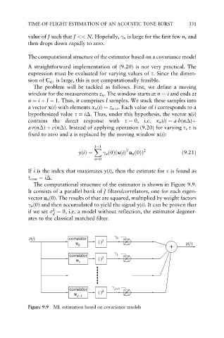
The computational structure of the estimator is shown in Figure 9.9.
It consists of a parallel bank of J filters/correlators, one for each eigen-
vector u n (0). The results of that are squared, multiplied by weight factors

n (0) and then accumulated to yield the signal y(i). It can be proven that
2
if we set ¼ 0, i.e. a model without reflection, the estimator degener-
d
ates to the classical matched filter.

γ
z(i) correlator 2 0
u ( ) y(i )
0 +
γ
correlator 2 1
u ( )
1

γ
correlator 2 J–1
u ( )
J–1
Figure 9.9 ML estimation based on covariance models