Page 49 - Classification Parameter Estimation & State Estimation An Engg Approach Using MATLAB
P. 49

38                               DETECTION AND CLASSIFICATION

            probabilities are given conditionally with respect to the true classes, i.e.
                def              def
                    !
            P miss ¼ P(^ ! 1 j! 2 ) and P fa ¼ P(^ ! 2 j! 1 ). In addition, we may define the prob-
                                     !
                                  def
            ability of a detection P det ¼ P(^ ! 2 j! 2 ).
                                       !
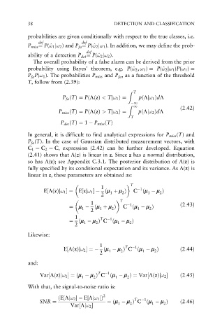
              The overall probability of a false alarm can be derived from the prior
                                                    !
                                                                !
            probability using Bayes’ theorem, e.g. P(^ ! 2 , ! 1 ) ¼ P(^ ! 2 j! 1 )P(! 1 ) ¼
            P fa P(! 1 ). The probabilities P miss and P fa , as a function of the threshold
            T, follow from (2.39):
                                                   Z  T
                         P fa ðTÞ¼ PðLðzÞ < Tj! 1 Þ¼   pðLj! 1 ÞdL
                                                     1
                                                     1                 ð2:42Þ
                                                   Z
                        P miss ðTÞ¼ PðLðzÞ > Tj! 2 Þ¼  pðLj! 2 ÞdL
                                                    T
                        P det ðTÞ¼ 1   P miss ðTÞ
            In general, it is difficult to find analytical expressions for P miss (T) and
            P fa (T). In the case of Gaussian distributed measurement vectors, with
            C 1 ¼ C 2 ¼ C, expression (2.42) can be further developed. Equation
            (2.41) shows that L(z) is linear in z. Since z has a normal distribution,
            so has L(z); see Appendix C.3.1. The posterior distribution of L(z)is
            fully specified by its conditional expectation and its variance. As L(z)is
            linear in z, these parameters are obtained as:
                                        1              1
                                                    T
                  E LðzÞj! 1 Š ¼  E½zj! 1 Š  ðm þ m Þ  C ðm   m Þ
                   ½
                                                               2
                                                          1
                                                2
                                            1
                                        2
                                                T
                                    1              1
                            ¼  m   ðm þ m Þ      C ðm   m Þ            ð2:43Þ
                                        1
                                                      1
                                            2
                                                           2
                                 1
                                    2
                              1         T   1
                            ¼ ðm   m Þ C ðm   m Þ
                                                   2
                                 1
                                               1
                                      2
                              2
            Likewise:
                                        1        T   1
                          E½LðzÞj! 2 м  ðm   m Þ C ðm   m Þ           ð2:44Þ
                                                2
                                                             2
                                                        1
                                           1
                                        2
            and:
                                       T   1
                Var LðzÞj! 1 Š ¼ ðm   m Þ C ðm   m Þ¼ Var LðzÞj! 2 Š   ð2:45Þ
                    ½
                                                          ½
                                              1
                                     2
                                 1
                                                  2
            With that, the signal-to-noise ratio is:
                                         2
                       ðE½Lj! 2 Š  E½Lj! 1 ŠÞ        T   1
                SNR ¼                     ¼ðm   m Þ C ðm   m Þ         ð2:46Þ
                                                            1
                                               1
                                                   2
                                                                2
                            Var½Lj! 2 Š
   44   45   46   47   48   49   50   51   52   53   54