Page 51 - Classification Parameter Estimation & State Estimation An Engg Approach Using MATLAB

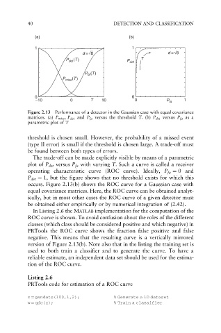
40 DETECTION AND CLASSIFICATION

(a) (b)
1 1
d =√8 d =√8
P det (T) P det T

(T)
P fa
P miss (T)

0 0
–10 0 T 10 0 P fa 1

Figure 2.13 Performance of a detector in the Gaussian case with equal covariance
matrices. (a) P miss , P det and P fa versus the threshold T. (b) P det versus P fa as a
parametric plot of T

threshold is chosen small. However, the probability of a missed event
(type II error) is small if the threshold is chosen large. A trade-off must
be found between both types of errors.
The trade-off can be made explicitly visible by means of a parametric
plot of P det versus P fa with varying T. Such a curve is called a receiver
operating characteristic curve (ROC curve). Ideally, P fa ¼ 0 and
P det ¼ 1, but the figure shows that no threshold exists for which this
occurs. Figure 2.13(b) shows the ROC curve for a Gaussian case with
equal covariance matrices. Here, the ROC curve can be obtained analyt-
ically, but in most other cases the ROC curve of a given detector must
be obtained either empirically or by numerical integration of (2.42).
In Listing 2.6 the MATLAB implementation for the computation of the
ROC curve is shown. To avoid confusion about the roles of the different
classes (which class should be considered positive and which negative) in
PRTools the ROC curve shows the fraction false positive and false
negative. This means that the resulting curve is a vertically mirrored
version of Figure 2.13(b). Note also that in the listing the training set is
used to both train a classifier and to generate the curve. To have a
reliable estimate, an independent data set should be used for the estima-
tion of the ROC curve.

Listing 2.6
PRTools code for estimation of a ROC curve

z ¼ gendats(100,1,2); % Generate a 1D dataset
w ¼ qdc(z); % Train a classifier