Page 50 - Classification Parameter Estimation & State Estimation An Engg Approach Using MATLAB

DETECTION: THE TWO-CLASS CASE 39

1
T
The quantity (m m ) C (m m ) is the squared Mahalanobis dis-
1 2 1 2
def ffiffiffiffiffiffiffiffiffiffip
tance between m and m with respect to C. The square root, d ¼ SNR
1
2
is called the discriminability of the detector. It is the signal-to-noise ratio
expressed as an amplitude ratio.
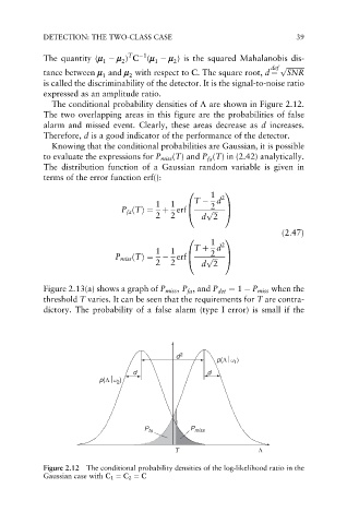
The conditional probability densities of L are shown in Figure 2.12.
The two overlapping areas in this figure are the probabilities of false
alarm and missed event. Clearly, these areas decrease as d increases.
Therefore, d is a good indicator of the performance of the detector.
Knowing that the conditional probabilities are Gaussian, it is possible
to evaluate the expressions for P miss (T) and P fa (T) in (2.42) analytically.
The distribution function of a Gaussian random variable is given in
terms of the error function erf():

1
0 1
T d 2
1 1
B 2 C
P fa ðTÞ¼ þ erf@ p ffiffiffi A
2 2 d 2
ð2:47Þ
1 2
0 1
1 1 T þ d
B 2 C
P miss ðTÞ¼ p
2
2 erf@ d 2
ffiffiffi A
Figure 2.13(a) shows a graph of P miss , P fa , and P det ¼ 1 P miss when the
threshold T varies. It can be seen that the requirements for T are contra-
dictory. The probability of a false alarm (type I error) is small if the

d 2
p(Λω )
1
d d
)
p(Λω 2

P fa P miss

T Λ

Figure 2.12 The conditional probability densities of the log-likelihood ratio in the
Gaussian case with C 1 ¼ C 2 ¼ C