Page 247 - Compression Machinery for Oil and Gas

Reciprocating Compressors Chapter 5 233

3
FEA
N = 6, D/d = 2.5
Griffith-Taylor
d = 8 in (203.2 mm)
2.5
Torsional stiffness ratio, K a /K b (–) 1.5 2

0.5 1

0
0 0.05 0.1 0.15 0.2 0.25 0.3 0.35 0.4
b/d (–)
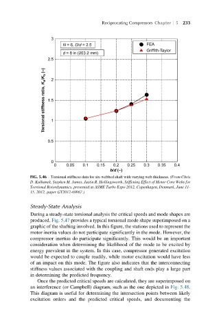
FIG. 5.46 Torsional stiffness data for six-webbed shaft with varying web thickness. (From Chris
D. Kulhanek, Stephen M. James, Justin R. Hollingsworth, Stiffening Effect of Motor Core Webs for
Torsional Rotordynamics, presented at ASME Turbo Expo 2012, Copenhagen, Denmark, June 11-
15, 2012, paper GT2012-69967.)

Steady-State Analysis
During a steady-state torsional analysis the critical speeds and mode shapes are
produced. Fig. 5.47 provides a typical torsional mode shape superimposed on a
graphic of the shafting involved. In this figure, the stations used to represent the
motor inertia values do not participate significantly in the mode. However, the
compressor inertias do participate significantly. This would be an important
consideration when determining the likelihood of the mode to be excited by
energy prevalent in the system. In this case, compressor generated excitation
would be expected to couple readily, while motor excitation would have less
of an impact on this mode. The figure also indicates that the interconnecting
stiffness values associated with the coupling and shaft ends play a large part
in determining the predicted frequency.
Once the predicted critical speeds are calculated, they are superimposed on
an interference (or Campbell) diagram, such as the one depicted in Fig. 5.48.
This diagram is useful for determining the intersection points between likely
excitation orders and the predicted critical speeds, and documenting the