Page 353 - Computational Fluid Dynamics for Engineers

11.6 Model Problem: Laminar and Turbulent Flat Plate Flow 343

- The top boundary velocities are specified and the pressure is extrapolated;
- The bottom boundary is specified on the flat plate, with zero pressure-
gradient normal to the wall. Symmetric flow is specified upstream of the
plate;
- The left boundary conditions are specified, and the normal velocity is ex-
trapolated from the interior;
- The right boundary pressure is specified, and the velocities are extrapolated.
The resulting program is included in Appendix B. Since the changes are
minimal, the program is not further discussed here, except that for commonality,
the eddy viscosity is computed for both laminar and turbulent flows. In the
former, the values are set to zero, whereas in the latter, they are obtained with
the Cebeci-Smith turbulence model.
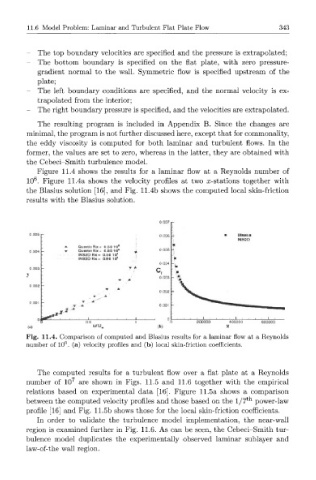
Figure 11.4 shows the results for a laminar flow at a Reynolds number of
6
10 . Figure 11.4a shows the velocity profiles at two x-stations together with
the Blasius solution [16], and Fig. 11.4b shows the computed local skin-friction
results with the Blasius solution.

Blflsais
INS2D
Qu»rticRx= 0.50 10* a
QUBrticRX- 0.80 10 ' * 0 005
INS2D flx= 0.50 10*
IN92D R x , 0.80 10 c -•
0004 7«
• A
0 003 _ i
• M.

^
u/U
(a) (b)
Fig. 11.4. Comparison of computed and Blasius results for a laminar flow at a Reynolds
6
number of 10 . (a) velocity profiles and (b) local skin-friction coefficients.

The computed results for a turbulent flow over a flat plate at a Reynolds
7
number of 10 are shown in Figs. 11.5 and 11.6 together with the empirical
relations based on experimental data [16]. Figure 11.5a shows a comparison
l
between the computed velocity profiles and those based on the / 7 t h power-law
profile [16] and Fig. 11.5b shows those for the local skin-friction coefficients.
In order to validate the turbulence model implementation, the near-wall
region is examined further in Fig. 11.6. As can be seen, the Cebeci-Smith tur-
bulence model duplicates the experimentally observed laminar sublayer and
law-of-the wall region.