Page 355 - Computational Fluid Dynamics for Engineers

11.7 Applications of INS2D 345

mental data. The models produced very similar results in most cases. Excellent
agreement between computational and experimental surface pressures was ob-
served, but only moderately good agreement was seen in the velocity profile
data. In general, the difference between the predictions of the different models
was less than the difference between the computational and experimental data.
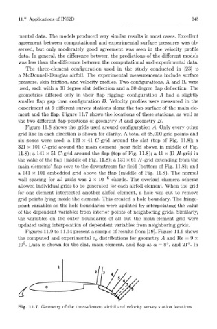
The three-element configuration used in the study conducted in [23] is
a McDonnell-Douglas airfoil. The experimental measurements include surface
pressure, skin friction, and velocity profiles. Two configurations, A and B, were
used, each with a 30 degree slat deflection and a 30 degree flap deflection. The
geometries differed only in their flap rigging: configuration A had a slightly
smaller flap gap than configuration B. Velocity profiles were measured in the
experiment at 9 different survey stations along the top surface of the main ele-
ment and the flap. Figure 11.7 shows the locations of these stations, as well as
the two different flap positions of geometry A and geometry B.
Figure 11.8 shows the grids used around configuration A. Only every other
grid line in each direction is shown for clarity. A total of 68,000 grid points and
six zones were used: a 121 x 41 C-grid around the slat (top of Fig. 11.8); a
321 x 101 C-grid around the main element (near field shown in middle of Fig.
11.8); a 141 x 51 C-grid around the flap (top of Fig. 11.8); a 41 x 31 #-grid in
the wake of the flap (middle of Fig. 11.8);al31x61 //-grid extending from the
main elements' flap cove to the downstream far-field (bottom of Fig. 11.8); and
a 141 x 101 embedded grid above the flap (middle of Fig. 11.8). The normal
wall spacing for all grids was 2 x 10 - 6 chords. The overlaid chimera scheme
allowed individual grids to be generated for each airfoil element. When the grid
for one element intersected another airfoil element, a hole was cut to remove
grid points lying inside the element. This created a hole boundary. The fringe-
point variables on the hole boundaries were updated by interpolating the value
of the dependent variables from interior points of neighboring grids. Similarly,
the variables on the outer boundaries of all but the main-element grid were
updated using interpolation of dependent variables from neighboring grids.
Figures 11.9 to 11.14 present a sample of results from [19]. Figure 11.9 shows
the computed and experimental c p distributions for geometry A and Re = 9 x
6
10 . Data is shown for the slat, main element, and flap at a = 8°, and 21°. In

Fig. 11.7. Geometry of the three-element airfoil and velocity survey station locations.