Page 45 - Computational Fluid Dynamics for Engineers

30 1. Introduction

0.04 0.04

0.02 0.02

y/c o.oo y/c o.oo

-0.02 h -0.02

1
. 0 . 0 4 '••• l - -- ' ' ' ' ' ' -0.04
-0.04
-0.04 -0.02 0.00 0.02 0.04 -C -0.02 0.00 0.02 0.04
x/c x/c
(a) (b)
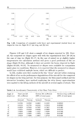
Fig. 1.30. Comparison of computed (solid lines) and experimental (dashed lines) ice
shapes for rime ice, flight 85-17: (a) wing, and (b) tail.

Figures 1.30 and 1.31 show a sample of ice shapes reported in [23]. Over-
all, the computed ice shapes agree well with the experimental data [26-28] in
the case of rime ice (flight 85-17). In the case of mixed ice at slightly higher
temperatures the calculation method still gives a good prediction of the ice
shape (flight 85-24a), although it does not predict the horns observed in flight
(flights 85-24b, 84-34). No measured ice shapes were available for comparison
under glaze ice conditions. However, it is expected that the measured ice shapes
would have exhibited multiple horns, which are difficult to predict.
In [23], studies were first conducted for the "clean" aircraft before studying
the effects of ice on the performance degradation of the aircraft for the computed
ice shapes on the wing and tail. For this purpose, the Hess panel method and the
interactive boundary layer method employing the strip theory approximation
were applied to the lifting surfaces of the aircraft at several angles of attack. The

Table 1.4. Aerodynamic Characteristic of the Clean Twin Otter.

Angle of Total aircraft Section lift coefficient Section drag coefficient
attack (a) lift coefficient (69% of semi-span) (69% of semi-span)

Inviscid Viscous Inviscid Viscous
0.4106 0.3516 0.4664 0.4334 0.00933
2° 0.6158 0.5716 0.6322 0.5910 0.00963
4° 0.8209 0.7615 0.7987 0.7457 0.01000
6° 1.0255 0.9509 0.9636 0.8909 0.01073
8° 1.2292 1.1209 1.1257 1.0238 0.01188
10° 1.4316 1.2405 1.2476 1.1504 0.01307
12° 1.6318 1.4388 1.4457 1.2719 0.01426