Page 175 - Computational Modeling in Biomedical Engineering and Medical Physics

164 Computational Modeling in Biomedical Engineering and Medical Physics

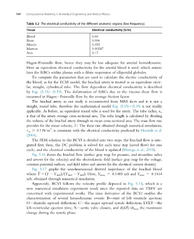
Table 5.2 The electrical conductivity of the different anatomic regions (low frequency).
Tissue Electrical conductivity [S/m]
Blood 0.66
Bone 0.006
Muscle 0.355
Marrow 0.00247
Arm 0.17

Hagen-Poiseuille flow, hence they may be less adequate for arterial hemodynamic.
Here an equivalent electrical conductivity for the arterial blood is used, which assimi-
lates the RBCs within plasma with a dilute suspension of ellipsoidal globules.
To compute the parameters that are used to calculate the electric conductivity of
the blood, as for the ECM model, the brachial artery is treated as an equivalent circu-
lar, straight, cylindrical tube. The flow dependent electrical conductivity is described
by Eqs. (5.15) (5.19). The deformation of RBCs due to the viscous shear flow is
measured in Hagen Poiseuille flow by the average friction factor.
The brachial artery in our study is reconstructed from MRI slices and it is not a
straight, round tube, therefore the mathematical model Eqs. (5.15) (5.19) is not readily
applicable. As before, an equivalent round tube is used for the artery. The tube radius, r 0 ,
is that of the artery average cross-sectional area. The tube length is calculated by dividing
the volume of the brachial artery through its mean cross-sectional area. The mass flow rate
provides for the mean velocity, U. The shear rate obtained through numerical simulations,
2
τ w . 0.1 N/m , is consistent with the electrical conductivity predicted by Hoetink et al.
(2004).
The FEM solution to the BCVI is divided into two steps: the brachial flow is inte-
grated first; then, the DC problem is solved for each time step (saved flow) for one
cycle, and the electrical conductivity of the blood is updated (Morega et al., 2018).
Fig. 5.16 shows the brachial flow (surface gray map for pressure, and streamline tubes
and arrows for the velocity) and the electrokinetic field (surface gray map for the voltage,
constant potential surfaces, and field tubes and arrows for the electrical current density).
Fig. 5.17 graphs the nondimensional derived impedance of the brachial blood
~
where Y 5 Y 2 Y min Þ= Y max 2 Y min Þ. Here, Y max 5 8.1481 mS and Y min 5 8.1414
ð
ð
mS, obtained through numerical simulation.
Apparently, BCVI follows the velocity profile depicted in Fig. 5.14, which is a
new numerical simulation experiment result since the reported data on TBEV are
concerned with experimental works. The time derivative of the BCVI enables the
characterization of several hemodynamic events: B—start of left ventricle ejection;
O—diastolic upward deflection; C—the major upward systole deflection; LVET—the
left-ventricular ejection time; X—aortic valve closure, and d(dZ)/dt max the maximum
change during the systole phase.