Page 170 - Computational Modeling in Biomedical Engineering and Medical Physics

Bioimpedance methods 159

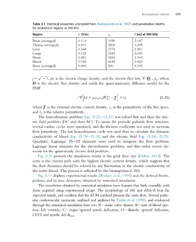
Table 5.1 Electrical properties (compiled from Andreuccetti et al., 1997) and penetration depths
for anatomical regions at 500 kHz.
Region σ [S/m] ε r δ [m] at 500 kHz

Brain (averaged) 0.110 1050 2.147
Thorax (averaged) 0.044 3000 3.395
Liver 0.148 2770 1.851
Lungs 0.123 1025 2.030
Heart 0.281 3265 1.343
Blood 0.748 4189 0.823
Bone (averaged) 0.006 200 9.193

p ffiffiffiffiffiffiffiffi
j 5 2 1, ρ V is the electric charge density, and the electric flux law, rUD ρ , where
5 v
D is the electric flux density and yields the quasi-stationary diffusion model for the
EMF
h i
e
2r σ 1 jωε 0 ε r ÞrV 2 J 5 0; ð5:25Þ
ð
e
where J is the external electric current density, ε 0 is the permittivity of the free space,
and ε r is the relative permittivity.
The hemodynamic problem Eqs. (5.21) (5.23) was solved first and then the elec-
tric field problem (DC and then AC). To attain the periodic pulsatile flow structure,
several cardiac cycles were simulated, and the friction coefficient was used to ascertain
flow periodicity. The last hemodynamic cycle was used then to calculate the dynamic
conductivity of blood Eqs. (5.15) (5.19) and the electric field Eqs. (5.24), (5.25).
Quadratic, Lagrange, P1 P2 elements were used to integrate the flow problem,
Lagrange linear elements for the electrokinetic problem, and first-order vector ele-
ments for the quasi-steady electric field problem.
Fig. 5.10 presents the simulation results at the peak flow rate (Dobre, 2012). The
aorta is the current path with the highest electric current density, which suggests that
the flow dynamics should be echoed by any fluctuation in the electric conductivity of
the aortic blood. This process is reflected by the bioimpedance, Z(t).
Fig. 5.11 displays experimental results (Woltjer et al., 1997) and the derived bioim-
pedance and its time derivative obtained by numerical simulation.
The waveforms obtained by numerical simulation have features that fairly resemble with
those acquired using experimental setups. The morphology of Z(t)and dZ(t)/dt bear the
expected trends, and confirms that the ECM method presents the aorta flow. Several partic-
ular cardiovascular moments, outlined and analyzed by Taylor et al. (1998),and evidenced
through the numerical simulation here too: X—aortic valve closure; B—start of blood ejec-
tion, left ventricle; C—major upward systole deflection; O—diastolic upward deflection,
LVET and systolic dZ/dt max .