Page 168 - Computational Modeling in Biomedical Engineering and Medical Physics

Bioimpedance methods 157

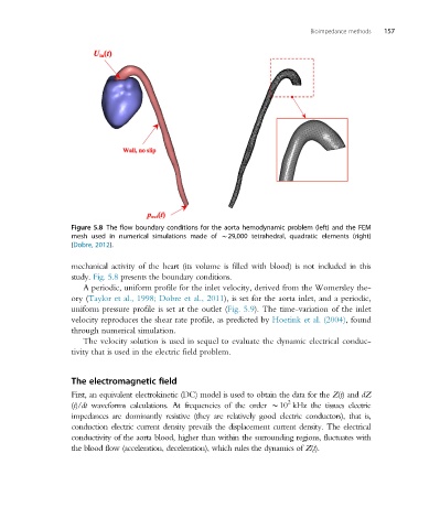
Figure 5.8 The flow boundary conditions for the aorta hemodynamic problem (left) and the FEM
mesh used in numerical simulations made of B29,000 tetrahedral, quadratic elements (right)
(Dobre, 2012).

mechanical activity of the heart (its volume is filled with blood) is not included in this
study. Fig. 5.8 presents the boundary conditions.
A periodic, uniform profile for the inlet velocity, derived from the Womersley the-
ory (Taylor et al., 1998; Dobre et al., 2011), is set for the aorta inlet, and a periodic,
uniform pressure profile is set at the outlet (Fig. 5.9). The time-variation of the inlet
velocity reproduces the shear rate profile, as predicted by Hoetink et al. (2004), found
through numerical simulation.
The velocity solution is used in sequel to evaluate the dynamic electrical conduc-
tivity that is used in the electric field problem.

The electromagnetic field

First, an equivalent electrokinetic (DC) model is used to obtain the data for the Z(t)and dZ
2
(t)/dt waveforms calculations. At frequencies of the order B10 kHz the tissues electric
impedances are dominantly resistive (they are relatively good electric conductors), that is,
conduction electric current density prevails the displacement current density. The electrical
conductivity of the aorta blood, higher than within the surrounding regions, fluctuates with
the blood flow (acceleration, deceleration), which rules the dynamics of Z(t).