Page 163 - Computational Modeling in Biomedical Engineering and Medical Physics

152 Computational Modeling in Biomedical Engineering and Medical Physics

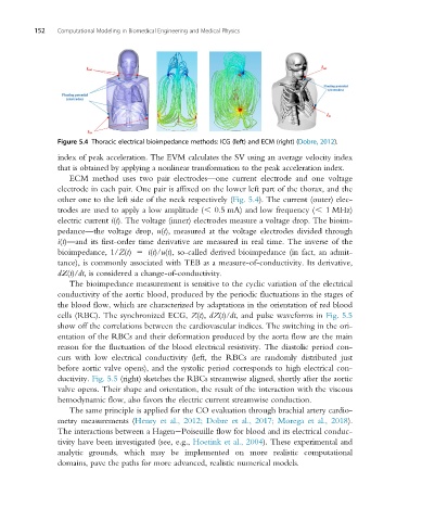
Figure 5.4 Thoracic electrical bioimpedance methods: ICG (left) and ECM (right) (Dobre, 2012).

index of peak acceleration. The EVM calculates the SV using an average velocity index
that is obtained by applying a nonlinear transformation to the peak acceleration index.
ECM method uses two pair electrodes—one current electrode and one voltage
electrode in each pair. One pair is affixed on the lower left part of the thorax, and the
other one to the left side of the neck respectively (Fig. 5.4). The current (outer) elec-
trodes are used to apply a low amplitude (, 0.5 mA) and low frequency (, 1 MHz)
electric current i(t). The voltage (inner) electrodes measure a voltage drop. The bioim-
pedance—the voltage drop, u(t), measured at the voltage electrodes divided through
i(t)—and its first-order time derivative are measured in real time. The inverse of the
bioimpedance, 1/Z(t) 5 i(t)/u(t), so-called derived bioimpedance (in fact, an admit-
tance), is commonly associated with TEB as a measure-of-conductivity. Its derivative,
dZ(t)/dt, is considered a change-of-conductivity.
The bioimpedance measurement is sensitive to the cyclic variation of the electrical
conductivity of the aortic blood, produced by the periodic fluctuations in the stages of
the blood flow, which are characterized by adaptations in the orientation of red blood
cells (RBC). The synchronized ECG, Z(t), dZ(t)/dt, and pulse waveforms in Fig. 5.5
show off the correlations between the cardiovascular indices. The switching in the ori-
entation of the RBCs and their deformation produced by the aorta flow are the main
reason for the fluctuation of the blood electrical resistivity. The diastolic period con-
curs with low electrical conductivity (left, the RBCs are randomly distributed just
before aortic valve opens), and the systolic period corresponds to high electrical con-
ductivity. Fig. 5.5 (right) sketches the RBCs streamwise aligned, shortly after the aortic
valve opens. Their shape and orientation, the result of the interaction with the viscous
hemodynamic flow, also favors the electric current streamwise conduction.
The same principle is applied for the CO evaluation through brachial artery cardio-
metry measurements (Henry et al., 2012; Dobre et al., 2017; Morega et al., 2018).
The interactions between a Hagen Poiseuille flow for blood and its electrical conduc-
tivity have been investigated (see, e.g., Hoetink et al., 2004). These experimental and
analytic grounds, which may be implemented on more realistic computational
domains, pave the paths for more advanced, realistic numerical models.