Page 252 - Computational Modeling in Biomedical Engineering and Medical Physics

Magnetic stimulation and therapy 241

Air
Fixator

Iron core Infinite
elements
Back plate
Coils

Tissue
Bone

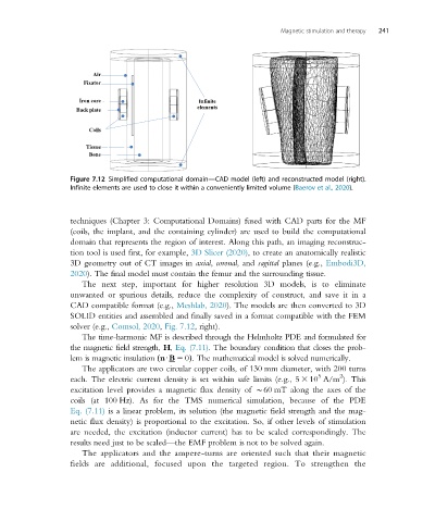
Figure 7.12 Simplified computational domain—CAD model (left) and reconstructed model (right).
Infinite elements are used to close it within a conveniently limited volume (Baerov et al., 2020).

techniques (Chapter 3: Computational Domains) fused with CAD parts for the MF
(coils, the implant, and the containing cylinder) are used to build the computational
domain that represents the region of interest. Along this path, an imaging reconstruc-
tion tool is used first, for example, 3D Slicer (2020), to create an anatomically realistic
3D geometry out of CT images in axial, coronal, and sagittal planes (e.g., Embodi3D,
2020). The final model must contain the femur and the surrounding tissue.
The next step, important for higher resolution 3D models, is to eliminate
unwanted or spurious details, reduce the complexity of construct, and save it in a
CAD compatible format (e.g., Meshlab, 2020). The models are then converted to 3D
SOLID entities and assembled and finally saved in a format compatible with the FEM
solver (e.g., Comsol, 2020, Fig. 7.12, right).
The time-harmonic MF is described through the Helmholtz PDE and formulated for
the magnetic field strength, H, Eq. (7.11). The boundary condition that closes the prob-
lem is magnetic insulation nUB 5 0ð Þ. The mathematical model is solved numerically.
The applicators are two circular copper coils, of 130 mm diameter, with 200 turns
5 2
each. The electric current density is set within safe limits (e.g., 5 3 10 A/m ). This
excitation level provides a magnetic flux density of B60 mT along the axes of the
coils (at 100 Hz). As for the TMS numerical simulation, because of the PDE
Eq. (7.11) is a linear problem, its solution (the magnetic field strength and the mag-
netic flux density) is proportional to the excitation. So, if other levels of stimulation
are needed, the excitation (inductor current) has to be scaled correspondingly. The
results need just to be scaled—the EMF problem is not to be solved again.
The applicators and the ampere-turns are oriented such that their magnetic
fields are additional, focused upon the targeted region. To strengthen the