Page 239 -

218 4 Feature detection and matching

s=0=1

t
x 0 x 0
ț
x(s)

s=0=1

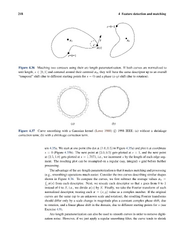
Figure 4.36 Matching two contours using their arc-length parameterization. If both curves are normalized to
unit length, s ∈ [0, 1] and centered around their centroid x 0 , they will have the same descriptor up to an overall
“temporal” shift (due to different starting points for s =0) and a phase (x-y) shift (due to rotation).

(a) (b)

Figure 4.37 Curve smoothing with a Gaussian kernel (Lowe 1988) c 1998 IEEE: (a) without a shrinkage
correction term; (b) with a shrinkage correction term.

ure 4.35a. We start at one point (the dot at (1.0, 0.5) in Figure 4.35a) and plot it at coordinate
s =0 (Figure 4.35b). The next point at (2.0, 0.5) gets plotted at s =1, and the next point
at (2.5, 1.0) gets plotted at s =1.7071, i.e., we increment s by the length of each edge seg-
ment. The resulting plot can be resampled on a regular (say, integral) s grid before further
processing.
The advantage of the arc-length parameterization is that it makes matching and processing
(e.g., smoothing) operations much easier. Consider the two curves describing similar shapes
shown in Figure 4.36. To compare the curves, we first subtract the average values x 0 =

x(s) from each descriptor. Next, we rescale each descriptor so that s goes from 0 to 1
s
instead of 0 to S, i.e., we divide x(s) by S. Finally, we take the Fourier transform of each
normalized descriptor, treating each x =(x, y) value as a complex number. If the original
curves are the same (up to an unknown scale and rotation), the resulting Fourier transforms
should differ only by a scale change in magnitude plus a constant complex phase shift, due
to rotation, and a linear phase shift in the domain, due to different starting points for s (see
Exercise 4.9).
Arc-length parameterization can also be used to smooth curves in order to remove digiti-
zation noise. However, if we just apply a regular smoothing filter, the curve tends to shrink