Page 243 -

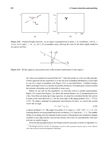
222 4 Feature detection and matching

y r max
(x i,y i) ș i
r
r i 0

-r max
x 0 ș 360
(a) (b)

Figure 4.42 Oriented Hough transform: (a) an edgel re-parameterized in polar (r, θ) coordinates, with ˆn i =
(cos θ i , sin θ i ) and r i = ˆn i · x i ; (b) (r, θ) accumulator array, showing the votes for the three edgels marked in
red, green, and blue.

y ^
n
l

d
ș x

Figure 4.43 2D line equation expressed in terms of the normal ˆn and distance to the origin d.

9
bin values are examined for potential line fits. Unless the points on a line are truly punctate,
a better approach (in my experience) is to use the local orientation information at each edgel
to vote for a single accumulator cell (Figure 4.42), as described below. A hybrid strategy,
where each edgel votes for a number of possible orientation or location pairs centered around
the estimate orientation, may be desirable in some cases.
Before we can vote for line hypotheses, we must first choose a suitable representation.
Figure 4.43 (copied from Figure 2.2a) shows the normal-distance (ˆn,d) parameterization for
a line. Since lines are made up of edge segments, we adopt the convention that the line normal
ˆ n points in the same direction (i.e., has the same sign) as the image gradient J(x)= ∇I(x)
(4.19). To obtain a minimal two-parameter representation for lines, we convert the normal
vector into an angle
θ = tan −1 n y /n x , (4.26)
√ √
as shown in Figure 4.43. The range of possible (θ, d) values is [−180 , 180 ] × [− 2, 2],
◦
◦
assuming that we are using normalized pixel coordinates (2.61) that lie in [−1, 1]. The number
of bins to use along each axis depends on the accuracy of the position and orientation estimate
available at each edgel and the expected line density, and is best set experimentally with some
test runs on sample imagery.
Given the line parameterization, the Hough transform proceeds as shown in Algorithm 4.2.

9 The Hough transform can also be generalized to look for other geometric features such as circles (Ballard
1981), but we do not cover such extensions in this book.