Page 247 -

226 4 Feature detection and matching

^
m i v
p i1
A
d 1
p i0

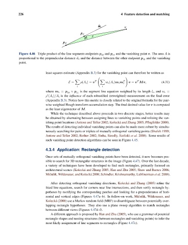
Figure 4.46 Triple product of the line segments endpoints p and p and the vanishing point v. The area A is
i0
i1
proportional to the perpendicular distance d 1 and the distance between the other endpoint p i0 and the vanishing
point.

least squares estimate (Appendix B.3) for the vanishing point can therefore be written as

T T T
E = ρ(A i )= v w i (A i )m i m v = v Mv, (4.31)
i
i i
where m i = p i0 × p i1 is the segment line equation weighted by its length l i , and w i =

ρ (A i )/A i is the influence of each robustified (reweighted) measurement on the final error
(Appendix B.3). Notice how this metric is closely related to the original formula for the pair-
wise weighted Hough transform accumulation step. The final desired value for v is computed
as the least eigenvector of M.
While the technique described above proceeds in two discrete stages, better results may
be obtained by alternating between assigning lines to vanishing points and refitting the van-
ishing point locations (Antone and Teller 2002; Koˇ seck´ a and Zhang 2005; Pflugfelder 2008).
The results of detecting individual vanishing points can also be made more robust by simulta-
neously searching for pairs or triplets of mutually orthogonal vanishing points (Shufelt 1999;
Antone and Teller 2002; Rother 2002; Sinha, Steedly, Szeliski et al. 2008). Some results of
such vanishing point detection algorithms can be seen in Figure 4.45.

4.3.4 Application: Rectangle detection

Once sets of mutually orthogonal vanishing points have been detected, it now becomes pos-
sible to search for 3D rectangular structures in the image (Figure 4.47). Over the last decade,
a variety of techniques have been developed to find such rectangles, primarily focused on
architectural scenes (Koˇ seck´ a and Zhang 2005; Han and Zhu 2005; Shaw and Barnes 2006;
Miˇ cuˇ s` ık, Wildenauer, and Koˇ seck´ a 2008; Schindler, Krishnamurthy, Lublinerman et al. 2008).

After detecting orthogonal vanishing directions, Koˇ seck´ a and Zhang (2005) refine the
fitted line equations, search for corners near line intersections, and then verify rectangle hy-
potheses by rectifying the corresponding patches and looking for a preponderance of hori-
zontal and vertical edges (Figures 4.47a–b). In follow-on work, Miˇ cuˇ s` ık, Wildenauer, and
Koˇ seck´ a (2008) use a Markov random field (MRF) to disambiguate between potentially over-
lapping rectangle hypotheses. They also use a plane sweep algorithm to match rectangles
between different views (Figures 4.47d–f).
A different approach is proposed by Han and Zhu (2005), who use a grammar of potential
rectangle shapes and nesting structures (between rectangles and vanishing points) to infer the
most likely assignment of line segments to rectangles (Figure 4.47c).