Page 246 -

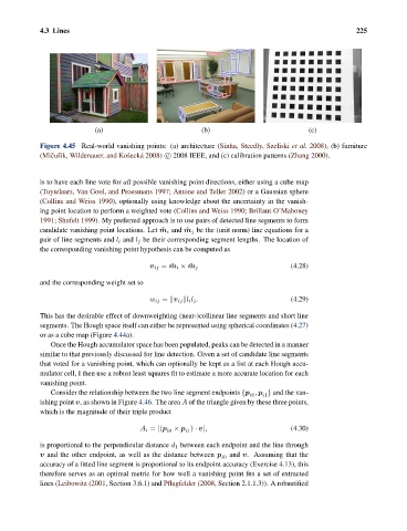
4.3 Lines 225

(a) (b) (c)

Figure 4.45 Real-world vanishing points: (a) architecture (Sinha, Steedly, Szeliski et al. 2008), (b) furniture
(Miˇ cuˇ s` ık, Wildenauer, and Koˇ seck´ a 2008) c 2008 IEEE, and (c) calibration patterns (Zhang 2000).

is to have each line vote for all possible vanishing point directions, either using a cube map
(Tuytelaars, Van Gool, and Proesmans 1997; Antone and Teller 2002) or a Gaussian sphere
(Collins and Weiss 1990), optionally using knowledge about the uncertainty in the vanish-
ing point location to perform a weighted vote (Collins and Weiss 1990; Brillaut-O’Mahoney
1991; Shufelt 1999). My preferred approach is to use pairs of detected line segments to form
candidate vanishing point locations. Let ˆm i and ˆm j be the (unit norm) line equations for a
pair of line segments and l i and l j be their corresponding segment lengths. The location of
the corresponding vanishing point hypothesis can be computed as

v ij = ˆm i × ˆm j (4.28)
and the corresponding weight set to

w ij = v ij l i l j . (4.29)

This has the desirable effect of downweighting (near-)collinear line segments and short line
segments. The Hough space itself can either be represented using spherical coordinates (4.27)
or as a cube map (Figure 4.44a).
Once the Hough accumulator space has been populated, peaks can be detected in a manner
similar to that previously discussed for line detection. Given a set of candidate line segments
that voted for a vanishing point, which can optionally be kept as a list at each Hough accu-
mulator cell, I then use a robust least squares fit to estimate a more accurate location for each
vanishing point.
Consider the relationship between the two line segment endpoints {p , p } and the van-
i0 i1
ishing point v, as shown in Figure 4.46. The area A of the triangle given by these three points,
which is the magnitude of their triple product

A i = |(p × p ) · v|, (4.30)
i0
i1
is proportional to the perpendicular distance d 1 between each endpoint and the line through
v and the other endpoint, as well as the distance between p i0 and v. Assuming that the
accuracy of a fitted line segment is proportional to its endpoint accuracy (Exercise 4.13), this
therefore serves as an optimal metric for how well a vanishing point fits a set of extracted
lines (Leibowitz (2001, Section 3.6.1) and Pflugfelder (2008, Section 2.1.1.3)). A robustified