Page 244 -

4.3 Lines 223

procedure Hough({(x, y, θ)}):
1. Clear the accumulator array.

2. For each detected edgel at location (x, y) and orientation θ = tan −1 n y /n x ,
compute the value of
d = xn x + yn y
and increment the accumulator corresponding to (θ, d).

3. Find the peaks in the accumulator corresponding to lines.
4. Optionally re-fit the lines to the constituent edgels.

Algorithm 4.2 Outline of a Hough transform algorithm based on oriented edge segments.

⇒

(a) (b)
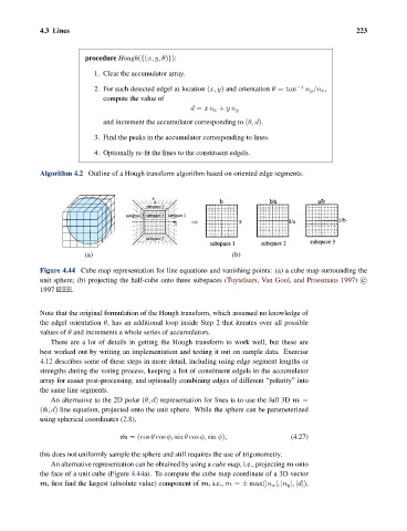
Figure 4.44 Cube map representation for line equations and vanishing points: (a) a cube map surrounding the
unit sphere; (b) projecting the half-cube onto three subspaces (Tuytelaars, Van Gool, and Proesmans 1997) c
1997 IEEE.

Note that the original formulation of the Hough transform, which assumed no knowledge of
the edgel orientation θ, has an additional loop inside Step 2 that iterates over all possible
values of θ and increments a whole series of accumulators.
There are a lot of details in getting the Hough transform to work well, but these are
best worked out by writing an implementation and testing it out on sample data. Exercise
4.12 describes some of these steps in more detail, including using edge segment lengths or
strengths during the voting process, keeping a list of constituent edgels in the accumulator
array for easier post-processing, and optionally combining edges of different “polarity” into
the same line segments.
An alternative to the 2D polar (θ, d) representation for lines is to use the full 3D m =
(ˆn,d) line equation, projected onto the unit sphere. While the sphere can be parameterized
using spherical coordinates (2.8),

ˆ m = (cos θ cos φ, sin θ cos φ, sin φ), (4.27)

this does not uniformly sample the sphere and still requires the use of trigonometry.
An alternative representation can be obtained by using a cube map, i.e., projecting m onto
the face of a unit cube (Figure 4.44a). To compute the cube map coordinate of a 3D vector
m, first find the largest (absolute value) component of m, i.e., m = ± max(|n x |, |n y |, |d|),