Page 242 -

4.3 Lines 221

(a) (b) (c)

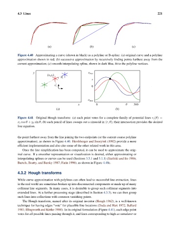
Figure 4.40 Approximating a curve (shown in black) as a polyline or B-spline: (a) original curve and a polyline
approximation shown in red; (b) successive approximation by recursively finding points furthest away from the
current approximation; (c) smooth interpolating spline, shown in dark blue, fit to the polyline vertices.

y r max
(x i,y i)
ș i
r
r i 0

-r max
x 0 ș 360
(a) (b)

Figure 4.41 Original Hough transform: (a) each point votes for a complete family of potential lines r i (θ)=
x i cos θ + y i sin θ; (b) each pencil of lines sweeps out a sinusoid in (r, θ); their intersection provides the desired
line equation.

the point furthest away from the line joining the two endpoints (or the current coarse polyline
approximation), as shown in Figure 4.40. Hershberger and Snoeyink (1992) provide a more
efficient implementation and also cite some of the other related work in this area.
Once the line simplification has been computed, it can be used to approximate the orig-
inal curve. If a smoother representation or visualization is desired, either approximating or
interpolating splines or curves can be used (Sections 3.5.1 and 5.1.1)(Szeliski and Ito 1986;
Bartels, Beatty, and Barsky 1987; Farin 1996), as shown in Figure 4.40c.

4.3.2 Hough transforms

While curve approximation with polylines can often lead to successful line extraction, lines
in the real world are sometimes broken up into disconnected components or made up of many
collinear line segments. In many cases, it is desirable to group such collinear segments into
extended lines. At a further processing stage (described in Section 4.3.3), we can then group
such lines into collections with common vanishing points.
The Hough transform, named after its original inventor (Hough 1962), is a well-known
technique for having edges “vote” for plausible line locations (Duda and Hart 1972; Ballard
1981; Illingworth and Kittler 1988). In its original formulation (Figure 4.41), each edge point
votes for all possible lines passing through it, and lines corresponding to high accumulator or