Page 287 -

266 5 Segmentation

(a) (b) (c)

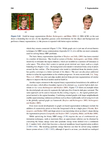
Figure 5.24 GrabCut image segmentation (Rother, Kolmogorov, and Blake 2004) c 2004 ACM: (a) the user
draws a bounding box in red; (b) the algorithm guesses color distributions for the object and background and
performs a binary segmentation; (c) the process is repeated with better region statistics.

which they remain connected (Figure 5.23b). While graph cuts is just one of several known
techniques for MRF energy minimization (Appendix B.5.4), it is still the one most commonly
used for solving binary MRF problems.
The basic binary segmentation algorithm of Boykov and Jolly (2001) has been extended
in a number of directions. The GrabCut system of Rother, Kolmogorov, and Blake (2004)
iteratively re-estimates the region statistics, which are modeled as a mixtures of Gaussians in
color space. This allows their system to operate given minimal user input, such as a single
bounding box (Figure 5.24a)—the background color model is initialized from a strip of pixels
around the box outline. (The foreground color model is initialized from the interior pixels,
but quickly converges to a better estimate of the object.) The user can also place additional
strokes to refine the segmentation as the solution progresses. In more recent work, Cui, Yang,
Wen et al. (2008) use color and edge models derived from previous segmentations of similar
objects to improve the local models used in GrabCut.
Another major extension to the original binary segmentation formulation is the addition of
directed edges, which allows boundary regions to be oriented, e.g., to prefer light to dark tran-
sitions or vice versa (Kolmogorov and Boykov 2005). Figure 5.25 shows an example where
the directed graph cut correctly segments the light gray liver from its dark gray surround. The
same approach can be used to measure the flux exiting a region, i.e., the signed gradient pro-
jected normal to the region boundary. Combining oriented graphs with larger neighborhoods
enables approximating continuous problems such as those traditionally solved using level sets
in the globally optimal graph cut framework (Boykov and Kolmogorov 2003; Kolmogorov
and Boykov 2005).
Even more recent developments in graph cut-based segmentation techniques include the
addition of connectivity priors to force the foreground to be in a single piece (Vicente, Kol-
mogorov, and Rother 2008) and shape priors to use knowledge about an object’s shape during
the segmentation process (Lempitsky and Boykov 2007; Lempitsky, Blake, and Rother 2008).
While optimizing the binary MRF energy (5.50) requires the use of combinatorial op-
timization techniques, such as maximum flow, an approximate solution can be obtained by
converting the binary energy terms into quadratic energy terms defined over a continuous
[0, 1] random field, which then becomes a classical membrane-based regularization problem
(3.100–3.102). The resulting quadratic energy function can then be solved using standard
linear system solvers (3.102–3.103), although if speed is an issue, you should use multigrid