Page 112 - Control Theory in Biomedical Engineering

98 Control theory in biomedical engineering

Given the nonlinear Hamiltonian (A.5) in the controls v and w, the process
of solving the OCP is to solve the state system (A.3) together with the
adjoint Eq. (A.6) and the following conditions:

∂HðtÞ ∂HðtÞ
∗
¼ ¼ 0at v ,w ∗ ðOptimality conditionsÞ
∂v ∂w (A.7)
T
λ ðt f Þ¼ 0 ðTransversality conditionÞ
OCPs are generally nonlinear and therefore generally do not have ana-
lytic solutions like the linear-quadratic OCP. As a result, it is necessary to
employ numerical methods to solve the OCP (A.1)–(A.7). The numerical
simulations are carried out by solving the state system (A.1) forward in time,
and the adjoint system (A.6) backward in time with the given optimality and
transversality conditions.

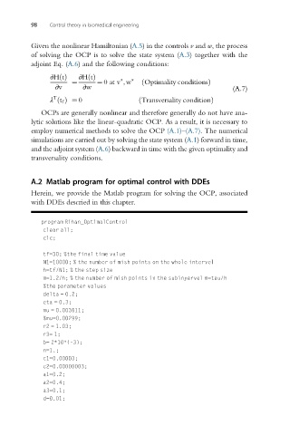
A.2 Matlab program for optimal control with DDEs

Herein, we provide the Matlab program for solving the OCP, associated
with DDEs descried in this chapter.

program Rihan_OptimalControl
clear all;
clc;

tf=30; %the final time value
N1=10000; % the number of mish points on the whole intervel
h=tf/N1; % the step size
m=1.2/h; % the number of mish points in the subinyervel m=tau/h
%the parameter values
delta = 0.2;
eta = 0.3;
mu = 0.003611;
%mu=0.00299;
r2 = 1.03;
r3= 1;
b= 2*10^(–3);
n=1.;
c1=0.00003;
c2=0.00000003;
a1=0.2;
a2=0.4;
a3=0.1;
d=0.01;