Page 133 - DSP Integrated Circuits

118 Chapter 4 Digital Filters

ripples have less significance than the width of the transition band. For example,
with 81 = 0.01 and §2 = 0.001, reducing any of the ripples by a factor of 2 increases
the filter order by only 6%. A decrease in the transition band by 50% will double
the required filter order. The required order for a bandpass filter is essentially
determined by the smallest transition band [1].
Deviations in the passbands and stopbands can also be expressed in terms of
maximum allowable deviation in attenuation in the passband, A max, and mini-
mum attenuation in the stopband,A mj n, respectively.

and

EXAMPLE 4.1

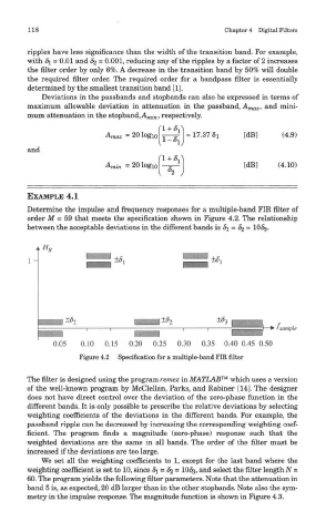
Determine the impulse and frequency responses for a multiple-band FIR filter of
order M = 59 that meets the specification shown in Figure 4.2. The relationship
between the acceptable deviations in the different bands is 5i = <% = 10^.

Figure 4.2 Specification for a multiple-band FIR filter

The filter is designed using the program remez in MATLAB™ which uses a version
of the well-known program by McClellan, Parks, and Rabiner [14]. The designer
does not have direct control over the deviation of the zero-phase function in the
different bands. It is only possible to prescribe the relative deviations by selecting
weighting coefficients of the deviations in the different bands. For example, the
passband ripple can be decreased by increasing the corresponding weighting coef-
ficient. The program finds a magnitude (zero-phase) response such that the
weighted deviations are the same in all bands. The order of the filter must be
increased if the deviations are too large.
We set all the weighting coefficients to 1, except for the last band where the
weighting coefficient is set to 10, since 81 = §2 = 10^, and select the filter length N =
60. The program yields the following filter parameters. Note that the attenuation in
band 5 is, as expected, 20 dB larger than in the other stopbands. Note also the sym-
metry in the impulse response. The magnitude function is shown in Figure 4.3.